How to Find Unique Values in Excel
(UNIQUE Function)
Not that it was impossible to find and sort out unique values in Excel – but yes, it was a task if not a hell of a task 🤕
Especially if it was to be done through functions. Before the introduction of the UNIQUE function, there wasn’t any function that allowed picking out unique values from a dataset so seamlessly.
Extracting values that occur only once, eradicating duplication, and filtering out a list of unique values through functions was something only Excel experts could do. But no more!
With the dynamic UNIQUE function of Excel, you can devise a simple formula to handpick unique values from a given dataset seamlessly. To learn all about doing this in Excel, get my free practice workbook for this guide here and read along with me till the end.
What does the UNIQUE function do
The UNIQUE function is a dynamic array function that returns an array of unique values from a given dataset.
For example, if you have a dataset cluttered with duplicate values. Supply it to the UNIQUE function along with the criteria of uniqueness 😎
The UNIQUE function will pick out the unique values from this dataset and return them as an array. You can supply it with any data (can be numbers, text, dates, etc.).
The UNIQUE function is only available in Microsoft 365 and Excel 2021. The previous versions of Excel do not support dynamic array functions.
Syntax
If you’re expecting the syntax of the UNIQUE function to be a long and complex one, sorry to burst your bubble but, it’s just about three arguments:
Array: The range or array from where the unique values are to be picked out.
By_Col: How is the data to be compared for uniqueness? If specified as 0 (FALSE), data is compared for uniqueness within columns, and unique columns are returned, and if specified as 1 (TRUE), unique rows are returned. It is an optional argument and defaults to 0 if omitted.
Exactly_Once: Which values are to be considered as unique? If set to 0 or omitted, it returns a set of all distinct values from a range. If set to 1, it only returns those values that appear in the data for once.
Return Value
The UNIQUE function returns an array (can be a column or a row) of unique values from a given dataset.
Since the result is going to be an array of values, it will spill across the neighboring cells (vertically or horizontally).
You’ll see plenty of them in the examples covered next ⬇
How to use the UNIQUE Function to find unique values
On to the juicy part – the examples 😃
We will now look into many use cases of the UNIQUE function.
By Rows
We have the names of some students arranged across a row in Excel.

There is some duplication in the names of students. To extract a list of unique names of students (excluding repetition), we will use the UNIQUE function.
Step 1) Write the UNIQUE function as follows:

Step 2) As the array argument, supply the cell range containing the student names.

Step 3) For the By_Col argument, we will give in 1 since we want the unique values to be found from a row (Row 2).

Step 4) Hit enter to get the list of unique values.

There are four unique names in Row 2. That’s how the UNIQUE function works for a row 💪
By Column
This example is a transpose of the one above. Just that the data is now arranged as columns and not rows.
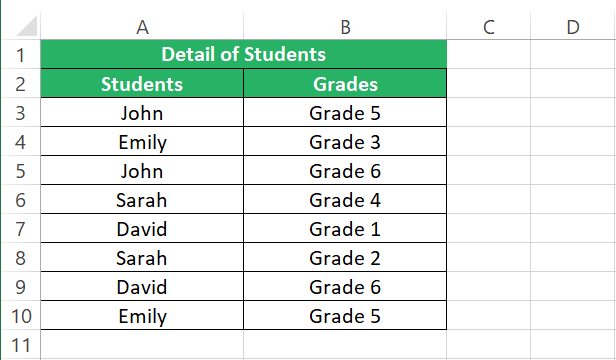
We now need to write the UNIQUE function to find out the unique student names from Column A (Cells A2:A10). For that:
Step 1) Write the UNIQUE function as follows:
Step 2) As the array argument, supply the cell range containing the student names i.e. A2:A10.
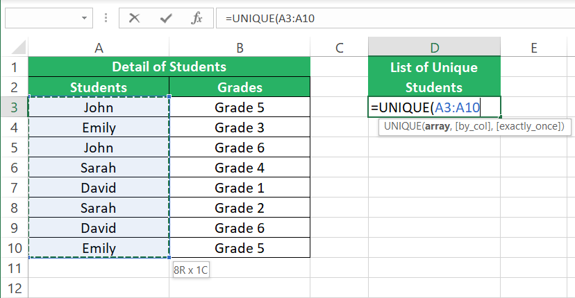
Step 3) This time we will leave the by_col argument omitted as we want the UNIQUE function to return unique values across the given column. It will default to 0.
Step 4) Hit enter to get the column of unique values.
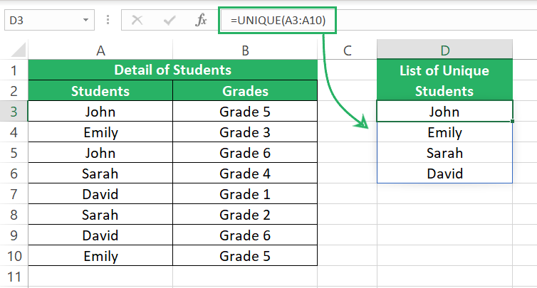
This time Excel produces a column of unique student names 🎯
Unique values that appear exactly once
In our dataset, we have instances of duplication of student names. Many names appear more than once.
As we apply the UNIQUE function to fetch a list of unique names, Excel pulls out a list with only one instance of each name 👩🏫
But what if I only want a list of those names that appear once (and not those that are duplicated or repeated more than twice)? For that, we will have to trigger the exactly_once argument.
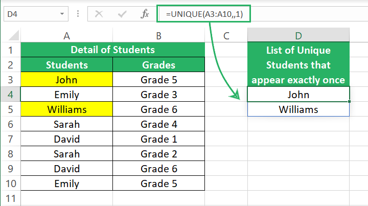
Step 1) To fetch a list of only those names that appear once, write the UNIQUE function as follows:
The array/cell range containing the names remains the same i.e. A3:A10.
Since we are running the search within a column, the by_col argument is omitted.
For the exactly_once argument, we have specified 1 / TRUE. This tells Excel that the parameter of “uniqueness” is “appearing exactly once”.
Step 2) Press enter to see the list of the student names that appear only once.
While you use the exactly_once argument, must know that if the supplied array doesn’t contain any instance of a value appearing exactly once, the UNIQUE function will return a #CALC! error.
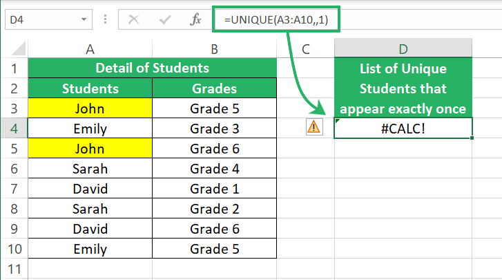
The data contains duplication of values, and all values appear more than once – so we get an error 👻
Unique values from multiple columns
You can also use the UNIQUE function across multiple columns at once.
For example, let’s now find a list of unique students from unique grades. This means we’d have to apply the UNIQUE function to multiple columns and not just to the student names column.
Step 1) To pull this list, write the UNIQUE function as follows:
The array/cell range includes cells from Column A (student names) and Column B (their grades).
Both the other arguments remain omitted.
Step 2) Press enter to see the Excel brings you.
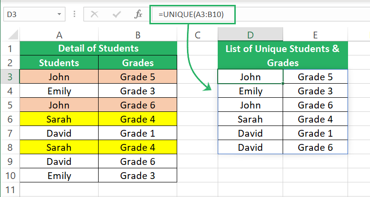
Look closely to see that the list produced by Excel contains duplication of names. For example, John appears twice, and so does David 👀
Paying some more attention reveals that this is because, for both the records of John, we have two different grades i.e., Grade 5 and 6. Hence, Excel treated both these records as distinct and included them in the list of unique values.
By contrary, Sarah is only included once in the list of unique values ❗
This is because in the original array, the student’s name Sarah, and the Grade 4 are the same in both instances. Excel therefore treats it as a duplication and includes it only once.
If I change the Grade for John to grade 5 for both instances in the source data, Excel will treat it as a duplication too, and include it only once.
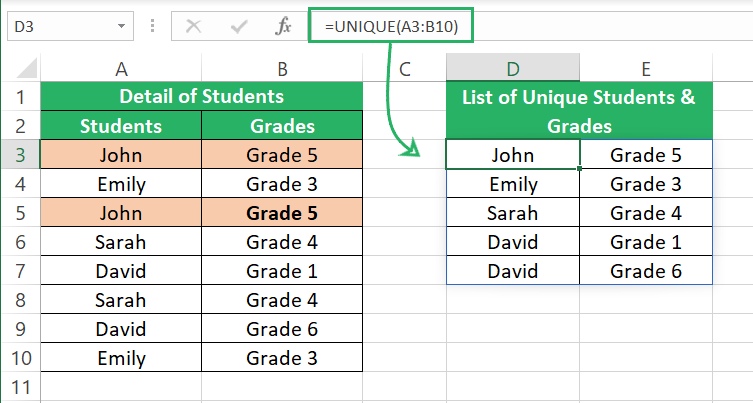
Hope this explains how the UNIQUE function works across multiple columns.
Troubleshooting the UNIQUE function
The UNIQUE function is an excellently thought and put-together dynamic array function. To make the most out of this function, make sure to bear the following pointers in mind 🔫
#SPILL! Error
Since the UNIQUE function is a dynamic array function, the result it produces would most probably be in an array (that spills across multiple neighboring rows and columns).
Make sure you have these rows and columns vacant. If any of these rows or columns are already occupied, the UNIQUE function will return a #SPILL! An error like below.
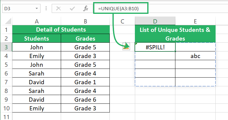
The array resulting from the UNIQUE function had to spill across the D3:E7 (the dotted blue line area). But as Cell E4 contains some text value (occupied cell), it obstructs the resulting array, and Excel returns the #SPILL! Error 💦
To help this situation, empty Cell E4 and the error would be replaced by the resulting array.
#NAME! Error
One of the many reasons why Excel returns the #NAME! error is when you make a spelling mistake while writing a function.
Often people would complain about this error when they try to write the UNIQUE function in Excel. This might be because you’re subscribed to an older version of Excel that doesn’t support/recognize the UNIQUE function.
Upgrade to Excel 2021 or Microsoft Office 365 to have access to this modern-day dynamic array function.
Deletion/Editing of formula
Click on the array where you have the results of the UNIQUE function populated, and you’ll see the same formula in the formula bar for all the cells (in a faded-out font though).
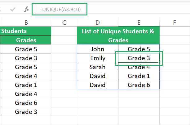
However, if you try to make changes to this formula, edit it, or delete it, Excel will either not allow you to do it or return the #SPILL! Error.
To make changes to the formula or delete it, click the cell that contains this function i.e., D3 in this case 📝
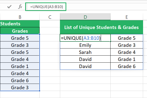
If you want to delete this formula anytime, activate the cell that contains it, and delete the formula from there. Or select the entire array and then delete it.
No other cell of the array would allow you to do this individually.
Conclusion
Dynamic array functions are the new flex of Microsoft Excel 365.
And why not – they rightly deserve to be. Array functions are designed to deal with large datasets quickly and efficiently. The UNIQUE function is an example. It can deal with huge sets of data to pick out the unique values based on the criteria you supply 💡
The result it produces is also an array. There are many dynamic array formulas in Excel, and if you want to learn more about what are they and how can you use them, read my following Advanced Excel tutorials.
