How to Hyperlink in Excel: Add, Edit, and Remove (Full Guide)

When you think of hyperlinks, you probably think of a link 🔗 that will direct you to a web page in one click.

While that is correct and cool, hyperlinks in Excel are way cooler!

Not only that they bring you to a specific file or a web page, but you can also insert hyperlinks to go to another cell or worksheet of the same workbook or even to another workbook🤯

Learn how to jump to cells or sheets or workbooks with hyperlinks in Excel!

Let’s jump in😀

Make sure to download your free practice workbook to work on as we go along.

Hyperlink to a website using the ribbon command

The most common hyperlinks that we know is the one that will direct you to a web page when you click a hyperlink text.

That’s exactly what you are going to learn first: How to insert a hyperlink to a website🌐

The most common way to insert a hyperlink in Excel is by clicking the Link button in the Insert Tab of the Excel Ribbon.

Open your practice workbook and let’s insert a hyperlink using the Excel ribbon command👇

1. Click on the cell. In our case, cell A1.
2. Click on the Insert Tab in the Excel ribbon.

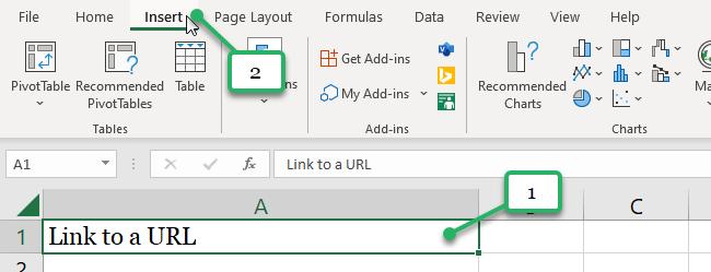
3. In the Links group, click Links or Hyperlinks (depending on your Excel version).

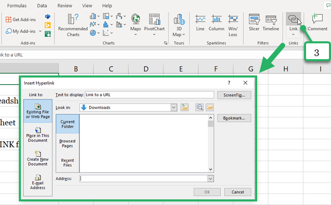
The Insert hyperlink dialog box will appear.

There may be a lot of things going on in this dialog box but you don’t have to worry. Let’s take things one step at a time😊

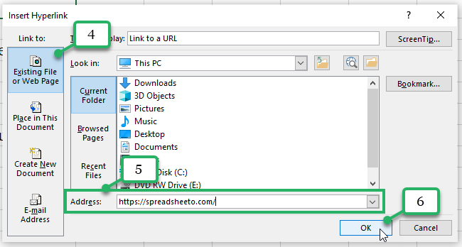
On the left side, you’ll see the Link to the panel which gives you options to link to Existing File or Web Page, Place in This Document, Create New Document, or E-mail Address.

4. Select Existing File or Web Page.
5. Add the URL (we will use https://spreadsheeto.com/) to the Address box at the bottom.
6. Finally, click OK.

The display text in the cell is now displayed in underlined blue color. This means that the text becomes a hypertext. Hypertext is text with hyperlinks.

Simply, a hyperlink🔗

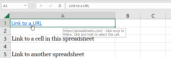
When you click the link, you will be directed to our Spreadsheeto main page🌐

Wasn’t that cool? Nice work👍

Pro Tip!

You can also use the Excel keyboard shortcut for inserting a link, Ctrl + K.

All you have to do is click on the specific cell and press the keys. Then the insert hyperlink dialog box will immediately appear (that’s why it’s our favorite).

This shortcut works in many apps too, so it’s good to know.

Hyperlink to a website by using right-click option

You can also add hyperlinks in Excel using the right-click option.

1. Right-click on the cell.
2. Click Link.

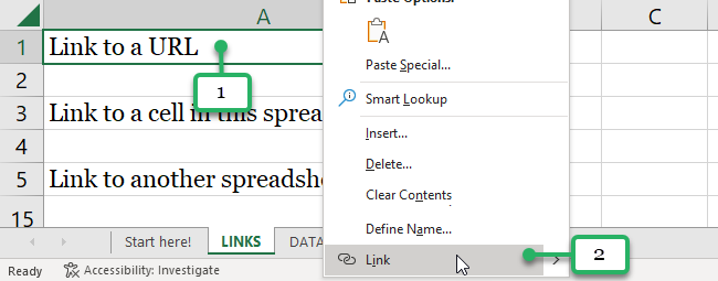
The Insert Hyperlink dialog box popup menu appears. You are going to make sure to click the Link to Existing File or Web Page option. Then add the URL in the Address and click OK.

The method will yield the same results. The cell becomes a hyperlinked cell😊

But did you know that Hyperlinks in Excel are not limited to only web pages? 🤯 You can insert hyperlinks to another cell within a worksheet, to another worksheet in the same workbook, or even to another Excel file.

And that’s exactly what you will learn next!

Hyperlink to another cell or worksheet

What makes Excel hyperlinks cooler is that you can insert a hyperlink to another cell or worksheet.

When dealing with a great amount of data in multiple worksheets, it can be super helpful to have a table of contents or summary report or a quick way to get from one commonly used section to another.

By using hyperlinks, you can know where this particular data is located in the workbook and directly access it by clicking the link.

You will appreciate this when you get to do it. So let’s go💪

1. Click on the cell (cell A3)
2. Press Ctrl + K to bring up the Insert Hyperlink dialog box.

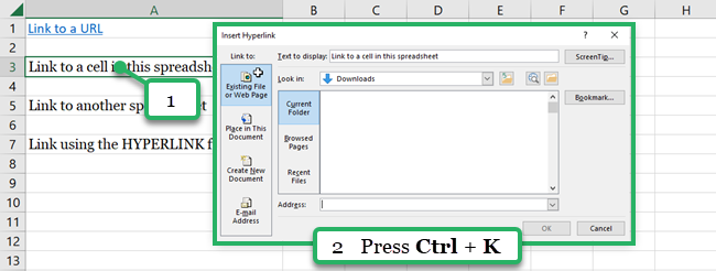
3. Select the Place in This Document option in the Link to the panel.

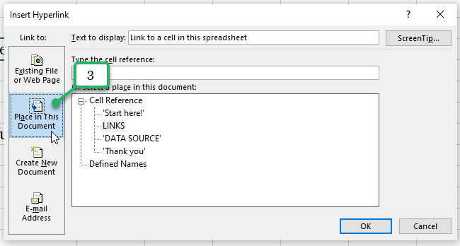
4. Under the cell reference, select the target worksheet in the same workbook. For our example, select Data Source Sheet.
5. Click OK to complete the formula.

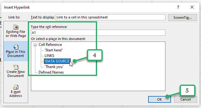
This is now the result.

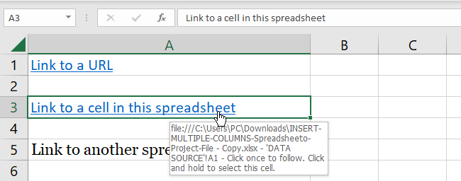
The text becomes a hyperlink. When you click the link, you will be directed to the Data Source worksheet in the current workbook.

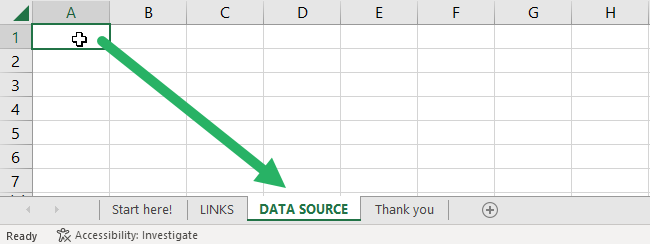
Link to a different workbook

You can also link to another excel workbook on your computer.

Let’s insert a link to another workbook in cell A5 of our practice workbook.

1. Click cell A5.
2. Press Ctrl + K.

The Insert hyperlink dialog box will appear. In the Link to the panel, click Excising File or Web Page option. Use the file explorer to find the file you want to link to.

Click any workbook file available on your computer. Then, click OK 👍

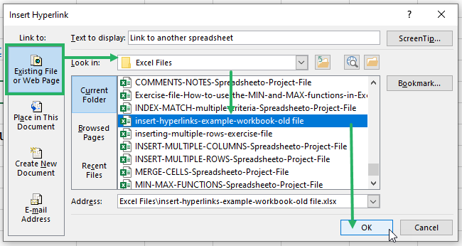
You have inserted a hyperlink that will direct you to another Excel file. When you hover over it, you can see the link destination.

Pro Tip!

It’s also possible to link to a specific cell in another file, but you’ll need to use the HYPERLINK function. I’ll show you how to do that in a few seconds.

How to remove hyperlinks

Removing hyperlinks is a two-click process. Whether you’ve added links that you don’t want anymore or that the links are irrelevant, you can remove hyperlinks very easily.

1. Right-click on the cell.
2. Select the Remove hyperlink option.

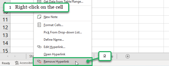
The hyperlink is now removed. The display text changed to black and won’t be able to direct you anywhere.ame column).

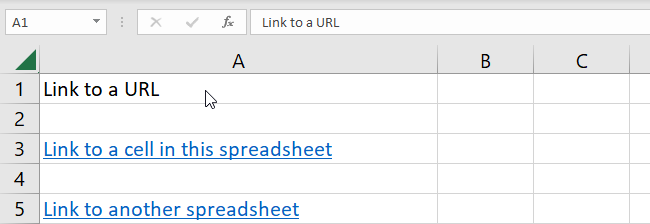
So easy, right?

How to edit a hyperlink

In the same way, you can edit a hyperlink using the right-click menu option.

Selecting cells to edit links can be tricky. When clicking the cell, you make click the link that will direct you to its link destination😬

To avoid that, you can Click and Hold on to that specific cell. When you see the pointer finger change to a cross, you can let go of the mouse button🖱️

This allows you to select the cell and edit it. To edit a hyperlink,

1. Click on the cell.
2. Right-click and select Edit Hyperlink.

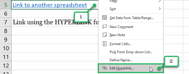
The edit hyperlink dialog box will appear. You can then edit your hyperlinks as you want. Whether you want to link to a new file or a web page, a cell, sheet, or workbook, you can do these steps to edit hyperlinks in Excel.

Hyperlink with the HYPERLINK function

As you know, Excel is a powerful spreadsheet program with lots of built-in functions to help you work efficiently with data and numbers. Excel has a function for inserting hyperlinks, too.

You can insert hyperlinks by using the HYPERLINK function in Excel.

The syntax of the HYPERLINK function is:

=HYPERLINK(link_location, [friendly_name])

The HYPERLINK function has the following arguments:

• link_location refers to a place in a document where the link points to. This could be a URL, a cell reference, or another spreadsheet or word file. This is required.
• friendly_name is the display text in the cell. It is displayed in blue and underlined. This is optional, but we recommend using it.

It makes for easier reading. If the friendly_name is omitted, the cell displays the link_location as the jump text.

The HYPERLINK function can be used in two important cases.

The first case is when you want to hyperlink to specific cells in external spreadsheets. The second case is when you want to hyperlink to a cell reference rather than using the URL.

Hyperlink function to cells in external spreadsheets

Let’s use this formula.

=HYPERLINK(“[name of the spreadsheet]cell reference”, “friendly name”)

For example, I want to link to a spreadsheet called “MIN-MAX-FUNCTIONS-Spreadsheeto-Project-File” and I want the link to point to cell B6 on the first sheet. Here’s how I’d do that:

=HYPERLINK(“[C:\Users\PC\Downloads\Excel Files\MIN-MAX-FUNCTIONS-Spreadsheeto-Project-File.xlsx]B6″,”Welcome!”)

Press Enter.

Instead of displaying the link location, a friendly name is displayed.

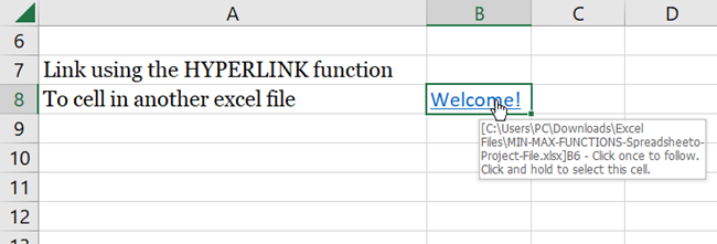
When you click the friendly name “Welcome!”, it will direct you to the cell reference of the Excel file.

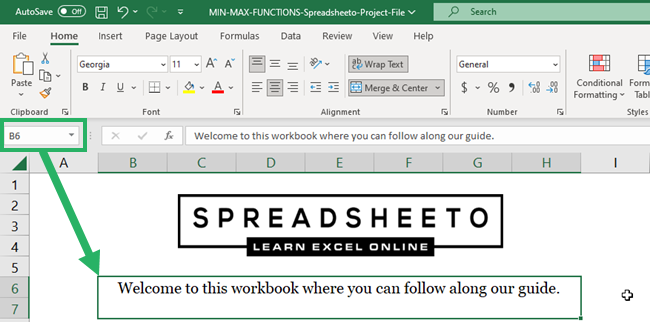
You just need to make sure to know the file location, the brackets, and the quotation marks are in the right place as well😊

Hyperlink function to cell reference

The second case in which you might want to use the HYPERLINK function is when the link could change.

In this case, you can use a cell reference instead of writing in the URL. This way, whenever the URL (or file path) in the cell changes, the link will automatically update.

For our example, the cell address of our URL is A12. So let’s type,

=HYPERLINK(A12,

For the friendly name, we can type anything, like “Website”.

Press Enter.

Even though the link in the cell address might change, the hyperlinked cell will automatically update.

How to find hyperlinks

You may find yourself working in a workbook that has links but you just can’t seem to find them. There is no automatic way to find all links in a workbook but there are several ways you can do to find them🧐

Whether you’re looking for workbook file names or links to another source, the best way is to determine the best search term to use.

To find links used in formulas, you can use Excel Find Feature🔍

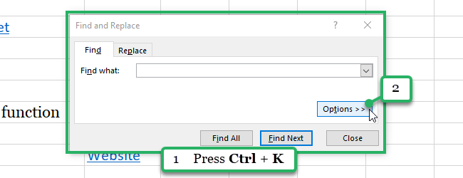
1. Press Ctrl + F on your keyboard to launch the Find and Replace dialog.
2. Click the Options button.

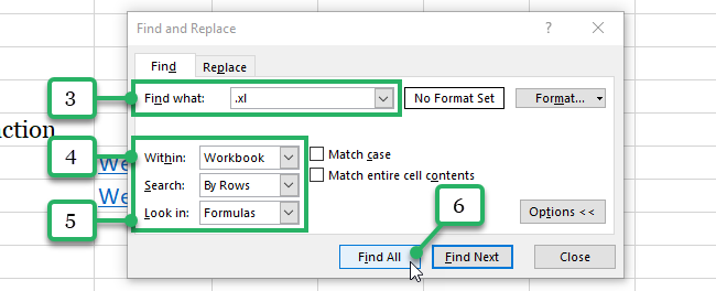
3. In the Find what box, type “.xl”
4. In the Within box, click Workbook.
5. In the Look in box, click Formulas.
6. Click Find All.

You will see the results below.

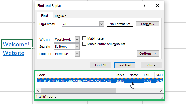
You can try to find other sources by using the best search term to use. You can also look in values, notes, and comments, not only in formulas.

That’s it – Now what?

Cool, right? Hyperlinks in Excel allow you to jump to different locations with a click!

Now, you know how to insert hyperlinks to direct you to either web pages or existing files. Plus, you also learned how to insert links to cells, sheets, or workbooks. Nice work👍

But wait, there’s more! You can level up how you navigate your way to cells, sheets, or workbooks in Excel when you learn advanced functions like IF, SUM, and VLOOKUP.

You’ll also learn how to effectively clean your data in Excel🚀

Join my free 30-minute video course and turbocharge your Excel skills!

Other resources

Looking up data across spreadsheets? Learn how to use the VLOOKUP function to find exactly what you need, fast.👑

Or you can read about one of the most versatile tools in Excel: Find and Replace here.

I hope this was helpful!

Frequently asked questions