Create a Table of Contents in Excel: Step-by-Step (2024)

In the world of data management, organization is key.

And what better way to keep track of all your valuable information than with a Table of Contents?

In this guide, we’ll show you how to create a Table of Contents in Excel that will help you stay on top of your data like a pro 💪

So get ready to take your spreadsheet game to the next level!

You can also download our sample workbook here to create an Excel table of contents.

Build a table of contents manually

Building a table of contents in an Excel sheet is easy. It might take you some time to understand it, but once you do, you will be able to navigate the sheet easily.

Let’s see how to do it below.

Say, we have a workbook that contains a couple of sheets. We want to create a TOC for all the sheets so we can directly access them from the first sheet 😃

To do that,

1. Identify the sheets in your document and decide which ones you want to include in the table of contents.
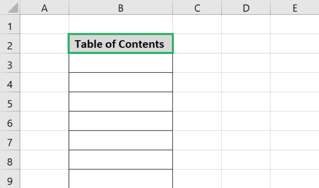
2. Create a new page at the beginning of the document where you want the table of contents to appear.
3. Type “Table of Contents” in cell B2.

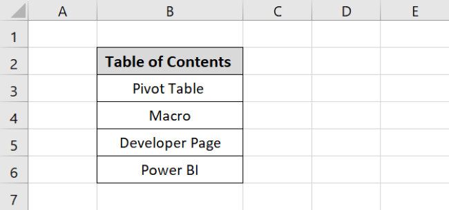
4. List the sheets you want to include in the table of contents.

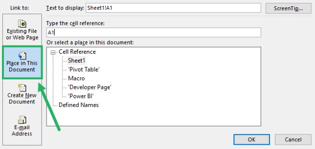
5. Now press CTRL + K on your keyboard or go to Insert Tab > Links to add the hyperlink.

The Insert Hyperlink dialog box appears.

6. Click Place in This Document.

7. Select the particular sheet name you want to reference in the cell.

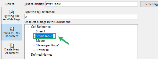
8. Press Ok.

The hyperlink will appear in the cell as:

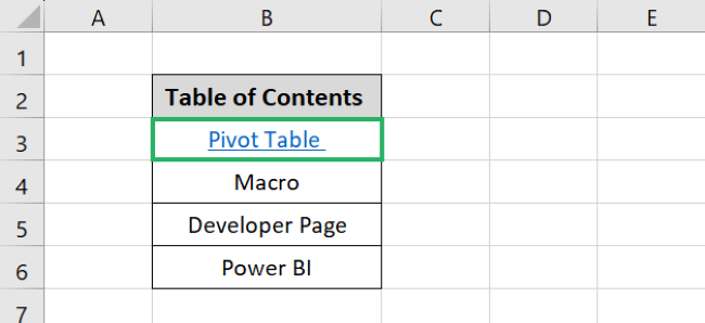
Clicking this will take you straight to the linked sheet, i.e., the Pivot Table.

Enter links in all cells for the corresponding worksheet.

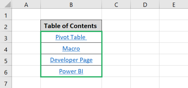
And it’s done. You can quickly access a certain sheet simply by clicking this link 🎯

Build a table of contents with a formula

Building a TOC using a formula is just as easy as creating it in a sheet manually. We will use the HYPERLINK function to link multiple sheets 🧐

Its syntax is given below.

=HYPERLINK(link_location, [friendly_name])

Where:

• link_location: the URL or cell reference to the hyperlink destination. This can be a file path, a web address, or a cell reference. If it is a cell reference, it must be enclosed in double quotes and include the sheet name (e.g., “#Sheet1!A1”).
• [friendly_name]: (optional) the text to display as the hyperlink. If omitted, the link_location will be displayed as the hyperlink text.

Let’s now see how to build a table of contents using a formula

To do that,

1. Type in Table of Contents on the first sheet of the workbook.

2. In cell B3, Enter the formula:

=HYPERLINK(

3. Enter the link location as

=HYPERLINK(“#Sheet2!A1”,

This means we want to reference cell A1 in sheet 2. If the sheet already has a name, the Hyperlink function will automatically convert it to that name 🤓

4. Enter the text you want to display as the hyperlink – we will enter Pivot Table.

=HYPERLINK(“#Sheet2!A1”, “Pivot Table”)

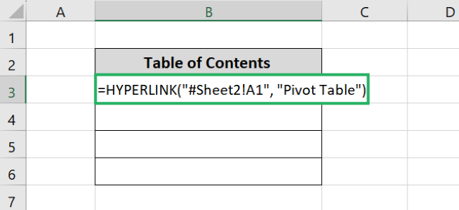
5. Press Enter.

And it’s done 🥇

The text containing the hyperlink appears in cell B3 as:

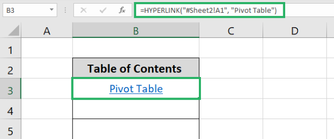
Do the same for the remaining cells, and you will have instant access to all sheets on one page.

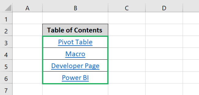
Pretty cool, no? 😎

That’s it – Now what?

In this article, we learned to create a table of contents. We saw how to build them manually as well as with formulas.

Having a TOC in your Excel workbook can make things a lot easier to understand. And with our easy-to-follow guide, you can now create a Table of Contents in Excel like a pro!

Not only will you reduce the risk of errors, but you will also be able to quickly locate the information you need 💻

So whether you’re managing large data or just want to organize data, Excel TOC can be helpful. Give it a try and see the difference it can make in your data management!

Also, try other important Excel functions like IF, SUMIF, VLOOKUP, etc. You can learn these functions for free in my 30-minute free email course. So sign up now!

Other resources

Did you enjoy reading this article? If yes, then you’d love to know more.

Try similar topics: How to Use Tables, Make a Data Table, Create a Pivot Table, and more.