Excel INDIRECT Function: Formulas and Examples (2024)
Some functions of Excel are simply meant to amaze you. The INDIRECT function is also one of that lot 🙈
Technically speaking, it will not perform any operation, nor will it run any logical tests to return Boolean Values. It is a unique function that’s different from all other functions of Excel.
If you have had too much suspense already, let’s just dive right into the guide below. What is the INDIRECT function, how is it used and what is it used for – we will answer that all in there. 👇
As you continue reading, do not forget to download our free sample workbook that’ll help you tag along with the guide.
Table of Contents
How to use the INDIRECT function
The INDIRECT crates an indirect reference to cells, ranges, sheets, and workbooks, too 🔄
Hard to get until we see an example of how it is applied, so here we go.
The image here has some value in Cell A2.

- Write A2 in another cell (Cell B2).
Make sure you don’t write it as =A2, or else Excel will create a link to Cell A2 in Cell B2. Right now, we are only writing A2 as a simple text ✍
- In another cell, write the INDIRECT function as follows:
= INDIRECT (B2)
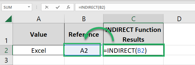
We have created a reference to Cell B2 (that contains the text string A2).
- Hit Enter.

Magic 💥 What’s that?
The Excel INDIRECT function returns the value of Cell A2.
From the backstage view, the INDIRECT function turned the text string in Cell B2 (A2) into a cell range and created an indirect reference to it.
So what if our data was not just a single cell but a column long like here 👀
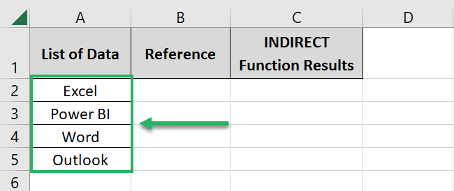
Not a problem!
- In Cell B2, write the cell range A2:A5.
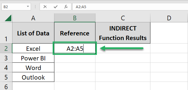
- Again write the INDIRECT function just like above.
= INDIRECT (B2)
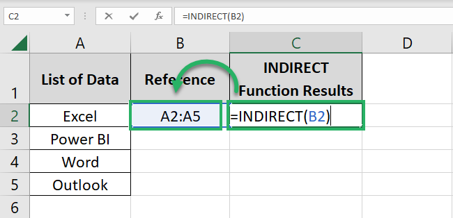
- Hit Enter.
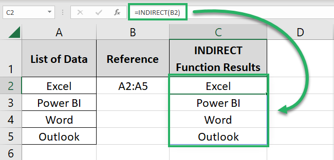
This time the INDIRECT function treats the text string A2:A5 as a range and returns the whole of it 😍
Pro Tip!
Whenever you delete, add, or move cells in Excel, it automatically updates the cell references in formulas.
The INDIRECT function doesn’t do that. For example, if you add a row before Column A in the example above, the column containing the data will move ahead and become Column B.
The INDIRECT function will not update the results and return the same cell range A2:A5 😎
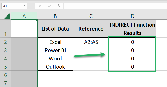
But how does it make sense to use it practically? We will see that in the examples below 💡
Other INDIRECT formula examples
We are on our way to more interesting examples of the INDIRECT function – you are sitting in tight, right?
Reference to other sheets (with and without CONCATENATE)
Using the INDIRECT function, you can not only create indirect references to other cells from the same sheet but to other sheets too.
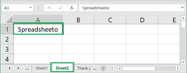
For example, here is Sheet 2 of an Excel workbook. Where Cell A1 contains a value 🚀
Pro Tip:
Note that when we create a reference to cells from other sheets, the reference looks like the below:
Sheet Name + Exclamation Mark (!) + Cell Reference
So, if we create a reference to Cell A1 from Sheet 2, it will look like this:
Sheet2!A1
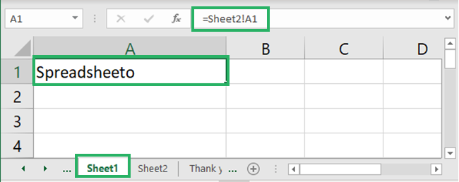
We are now in Sheet 1 of the same workbook. To create an indirect reference to Cell A1 from Sheet2:
- Activate a cell (Cell A2) and write the sheet reference below:
Sheet2!A1
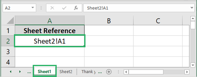
- In another cell, write the INDIRECT function as follows:
= INDIRECT (A2)
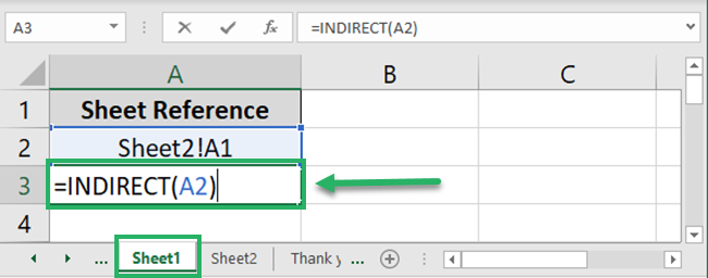
- Hit Enter and you have your indirect reference to another sheet all set ✌
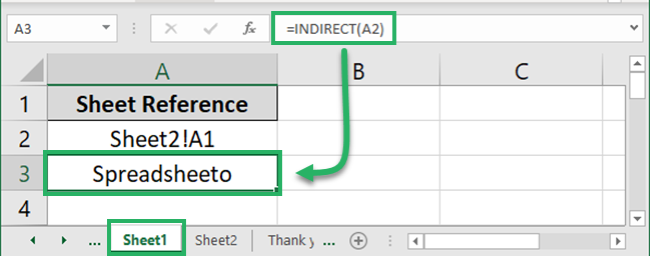
We have the value from cell A1 of Sheet 2 in Sheet 1. Yay!
If you find it hard to write the cell reference from another sheet like that, you may use the CONCATENATE function as below:
- Write the name of the sheet and cell reference in different cells. And merge them with an exclamation mark in between to get the sheet reference like below.
= CONCATENATE (A2,”!”, B2)

Must not forget to enclose the exclamation mark in double quotation marks 🗯
- Wrap the above function in the INDIRECT function.
= INDIRECT (CONCATENATE (A2,”!”, B2))

- Hit Enter to reach the same results again.
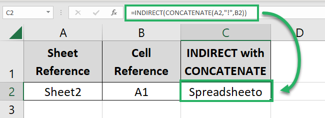
Fun, isn’t it 🍭
Performing functions on Named Ranges
The INDIRECT function can not only recognize cell references and ranges but named ranges too. See for yourself.
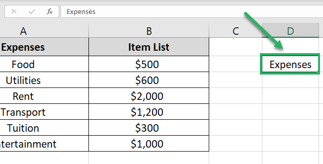
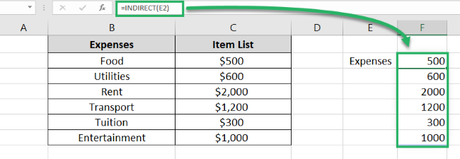
Here is a list of some expenses (yeah, many of them) 💰
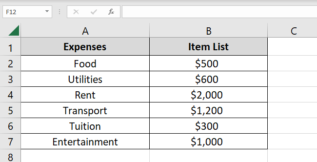
Turn them into a named range by following these steps:
- Select the list of expenses (the numbers only).
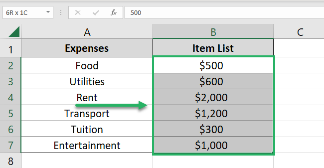
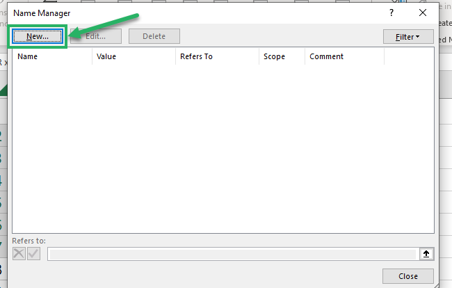
- Go to the Formulas tab > Name Manager.

- From the Name Manager dialog box, select New.
- Set a name for the defined range (we are setting it to Expenses).
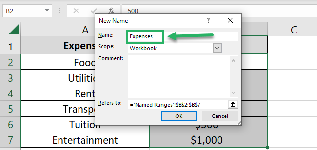
- Click Okay.
The range is saved by the name Expenses 🎯
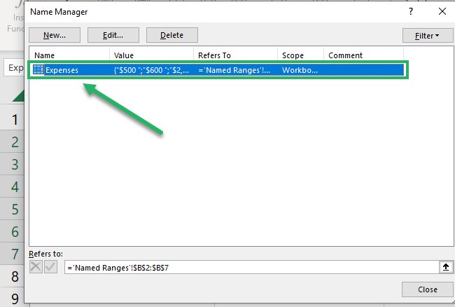
- Close the Name Manager.
- Activate any cell (Cell D2) and write the name of the range (Expenses) in it. Make sure not to make any spelling mistakes.
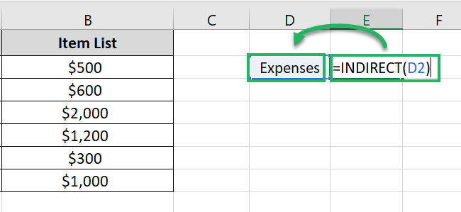
- In another cell write the INDIRECT function as follows:
= INDIRECT (D2)
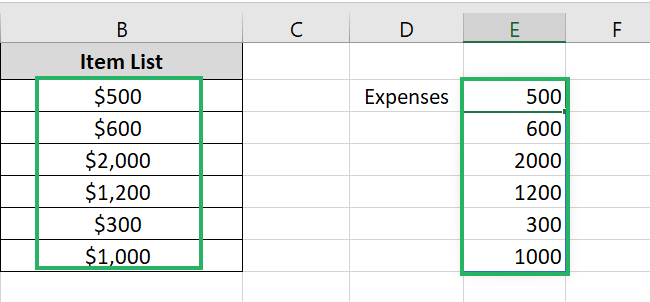
- Hit Enter to see that the INDIRECT function will return the whole range that you saved by the name Expenses 💁♀️
Cool! But we will take it a step ahead.
- Now wrap the INDIRECT function in the SUM function as below:
= SUM (INDIRECT (D2))
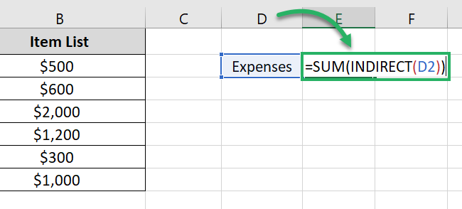
- Hit Enter.
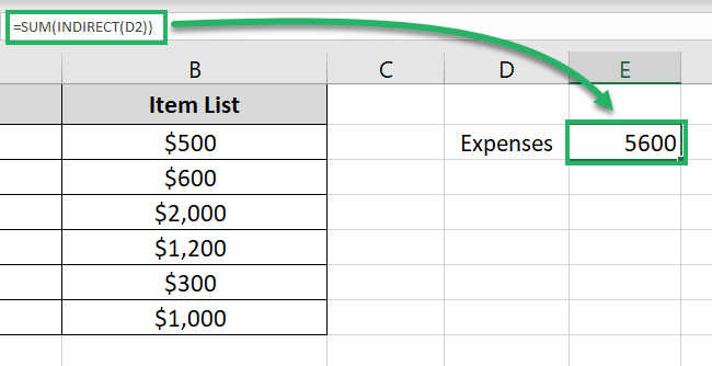
Viola! We have the sum of the range Expenses. That’s how you can use the INDIRECT function to create an indirect reference to ranges 💪
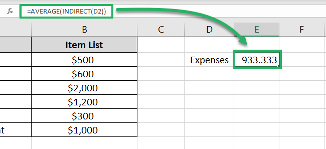
You may try any function with that. For example, wrap the INDIRECT function above in the AVERAGE function to get the average of the said range.
= AVERAGE (INDIRECT (D2))
Pro Tip!
Named ranges are not like cell references.
Even if you add, move or delete cells before or after a named range (Expenses), the answer to the INDIRECT function won’t change. See that below 🚴♂️
- Add a column behind Column A as below
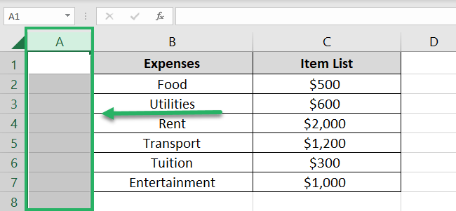
- The answer to the INDIRECT function remains unchanged. That’s because the range of Expenses remains unchanged 🏆
That’s it – Now what?
Through the above guide, we have learned the primary use and operation of the INDIRECT function in Excel.
Not to forget, we have also seen multiple examples of you can bring it to use practically. Hope you enjoyed learning about it 🧐
Because if you did, your learning journey has yet only begun. There are so many more functions in the Excel library that you must explore.
To begin with, I suggest you learn about the VLOOKUP, SUMIF, and IF functions (my top favorite Excel functions).
Other resources
The INDIRECT function can only create an indirect reference to another cell. But how do you create a direct reference in Excel?
There are three kinds of direct references that you can create in Excel – learn about them all here.
