Excel ISNA Function Guide: How and When to Use
So you have taken all your time to write a lookup function. But as you hit Enter, instead of the desired value, all that you get in return is the #N/A error.
Duhh… 🥴
A function or a formula returns the #N/A error in Excel when it fails to find the value it has been asked for. No matter how distasteful it looks, you will face the #N/A function in Excel very often. Especially if you use the lookup functions 🙈
But that’s alright – We have the ISNA function in Excel to handle the #N/A errors. To know all about the ISNA function of Excel, jump straight into the guide below.
And yeah, download our free sample workbook here to tag along with the guide.
Table of Contents
How to use the ISNA function in Excel
Using the ISNA function in Excel is literally the easiest. You only need to write the ISNA function and refer to the cell or the formula that you want to be checked for the #N/A error.
For example, check here.
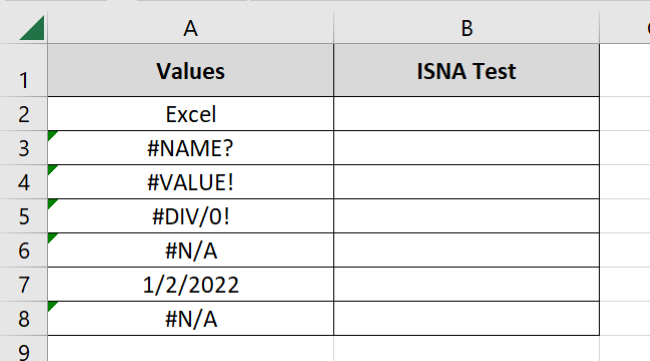
The above image has a list of values. Some are error values, and others are formulas or values.
You can use the ISNA function to check each of these cells – do they contain the N/A error? Let’s do it together here 👇
- In the first cell, write the ISNA function as follows:
= ISNA (A2)
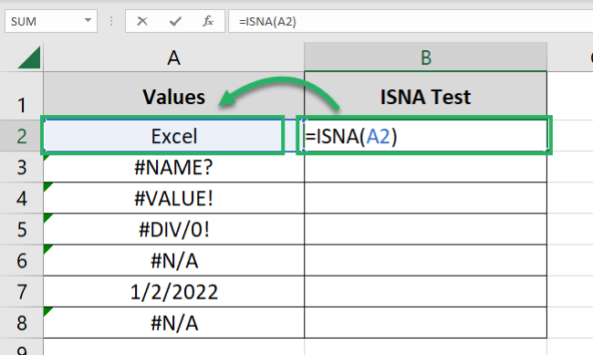
- Hit Enter, and that’s it.
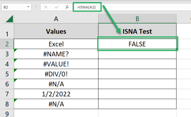
- Drag and drop the same formula to the whole list. Here come the results:
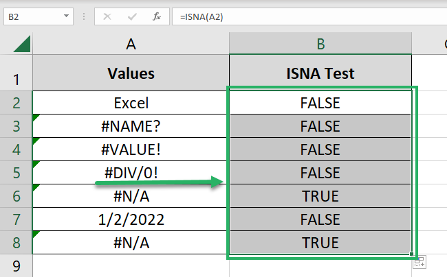
For all those cells that have the #N/A error, we get TRUE. And for all the cells with any other value, the ISNA function returns FALSE.
Using the ISNA function alone in Excel makes little sense. However, it becomes super useful when used together with other functions of Excel to evaluate a formula.
Excel ISNA VLOOKUP formula example
The VLOOKUP function is one of Excel’s most commonly known (and used) lookup functions 🔍
It looks for a given lookup value in the first column of a lookup range and returns the corresponding value from any row of that range.
For example, here:
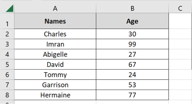
The image above has a list of age records extracted from the national database (let’s assume that 😜).
Below, we have a list of people (on the right) whose ages we want to extract from the list on the left.
- For that, write the VLOOKUP function as follows:
=VLOOKUP(D2,$A$2:$B$8,2,0)
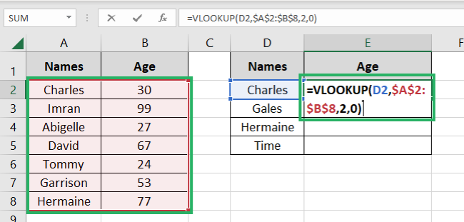
- D2 contains the lookup value (Charles). The person whose age is sought.
- $A$2:$B$8 contains the table array from where the lookup value is sought.
- 2 tells the column number in the table array from where this value is sought. We need the age, so we have referred to column 2 (Ages).
- 0 represents the exact match mode. We do not want VLOOKUP to return approximate matches.
Note that we have turned the table array reference into an absolute one ($A$2:$B$8). This is because we will drag drown this formula to the whole list later👀
And we don’t want Excel to change the cell reference for the table array when we do that.
- All good? Hit Enter to get the results as follows:
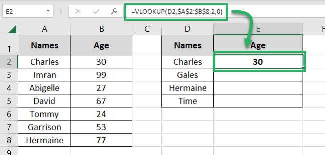
We get the age of Charles from the table array – that’s 30. But some names in the list (on the right side), might not be present in the list (on the left side) 🤔
How will the VLOOKUP function find the ages for such names? Let’s see that below.
- Drag and drop the same formula to the entire list of names.
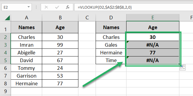
There are the results. For the names present in the list (on the left side), the VLOOKUP returns the age of the people 🧓
But for the names missing from there, we get the #N/A error. Is there some way we can avoid this error?
The ISNA function can help you do that. For that:
- Wrap the VLOOKUP function in the ISNA function as follows:
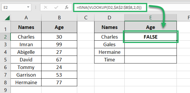
=ISNA(VLOOKUP(D2,$A$2:$B$8,2,0))

- Hit Enter to see the results for yourself.
- Drag and drop the same to the whole list as follows:
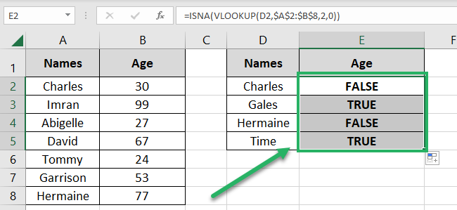
What has the ISNA function done? It evaluates the VLOOKUP function for the #N/A error. If the VLOOKUP function results in an error – the ISNA returns TRUE ✅
And if not, the ISNA function returns FALSE.
This can help you know which name would return an #N/A error beforehand. Accordingly, you can amend your function to prevent the #N/A error.
Excel IF ISNA formula Example
Using the ISNA function with other functions can help you evaluate an #N/A error. But how can you fix this error?
For that, you need to use the IF function together with ISNA. How? Check it out here 🚀
In the example above, we have the TRUE and FALSE values for where there is or there is not an #N/A error. But now we want to replace them with results.
So what do we exactly want to do?
- We want the VLOOKUP function to return the age where the name exists in the table array.
- And if the name doesn’t exist in the table array, we want the value “No Record Found” returned.
To do this, we need to use the ISNA and IF functions together as below 📌
- Wrap the VLOOKUP function in the ISNA function.
=ISNA(VLOOKUP(D2,$A$2:$B$8,2,0))
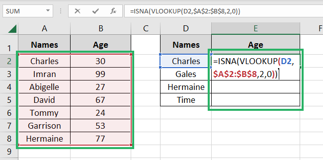
- Wrap the above function in the IF Function as follows:
= IF ( ISNA ( VLOOKUP ( D2, $A$2:$B$8, 2,0 ) ),
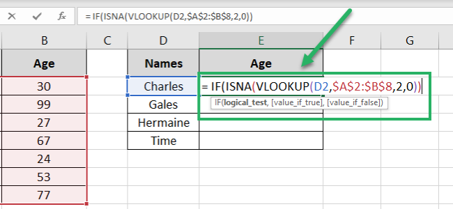
Until now, we have only nested the above formula in the IF function 🎁
- Write the value_if_true argument for the IF function.
= IF ( ISNA ( VLOOKUP ( D2, $A$2:$B$8, 2,0 ) ), “No Record Found”
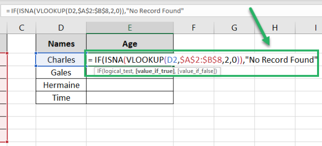
The IF function returns the value_if_true if the answer of the ISNA function comes out TRUE. And the ISNA function would return TRUE when the VLOOKUP function returns the #N/A error 📍
This means the #N/A error to be posed by the VLOOKUP function would now be replaced by the value “No Record Found”.
- Write the value_if_false argument for the IF function.
=IF(ISNA(VLOOKUP(D2,$A$2:$B$8,2,0)),”No Record”,VLOOKUP(D2,$A$2:$B$8,2,0))
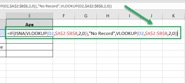
So at this stage, here’s the summary of what would happen📝
The above function would return:
- “No Record Found” if the VLOOKUP fails to find the given name in the table array; and
- The age of the person if the VLOOKUP finds the given name in the table array.
- Hit Enter, and that’s it.
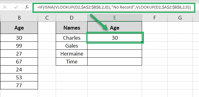
- Drag and drop the same to the whole list.

Yay! We no more have any unpleasant #N/A errors on our list. Either we have the age of the given person or the value specified by us 🏆
That’s it – Now what
And here the ISNA function comes to an end. It is one of the simplest functions of Excel that only performs a logical test and returns a Boolean value (True or False).
The ISNA function can become all the more useful if used together with other functions from the super big functions library of Excel 💪
While all the functions of Excel are equally useful, there are some functions that one must master. Like the VLOOKUP, SUMIF, and IF functions.
Don’t worry if you’re not good at them already. My 30-minute free email course will take you through them all. To enroll, click here now.
Other resources
If you enjoyed reading about the ISNA function, you’d love to know about its twin – the ISERROR function.
The ISNA function only checks for #N/A errors. Whereas the ISERROR function performs the same job for literally all kinds of errors in Excel.
Learn about the ISERROR and IFERROR functions of Excel here.
