How to Refresh a Pivot Table in Excel

Pivot table is a powerful Excel tool that lets you analyze, transform and present large data sets in a concise and composed manner 📄

However, working with large datasets often requires tweaks like applying a different formula or adding more details. This change made in the dataset is not directly reflected in your pivot table.

To do that, you need to refresh your pivot table so it can project the changes made in your dataset on the pivot table. We will see different methods of doing that in this guide.

Download our sample workbook here to practice refreshing a pivot table in Excel 😃

Table of Contents

What is a pivot table?

Before we get into the how of refreshing a pivot table, let’s first take a brief look at what a pivot table is and how refreshing a pivot table works.

A pivot table is a highly interactive and useful feature in Excel that lets you transform raw data into a meaningful form. You can summarize, filter, organize and present large data neatly 🔍

Refreshing a pivot table is necessary because when you create a pivot table, it is based on a certain data range that is stored in the pivot cache.

If you make any changes to the dataset, they are not reflected in the pivot table. When you refresh the pivot table, Excel updates it with the latest dataset in the given range 💻

This ensures any changes you made in the original dataset are accurately displayed in your pivot table. There are different ways you can refresh a pivot table, from manually updating to automating.

Let’s learn all these methods below.

Refresh a pivot table using ribbon in Excel

The most common way of refreshing your pivot Excel table is using ribbon. Let’s see how to do that.

Say, we have the following sample dataset.

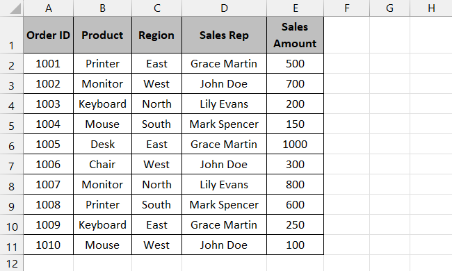
Its pivot table is as follows. We will change some values in our dataset and refresh the pivot table to see if the changes appear or not 📑

To do that,

Step 1) Click on the pivot table to activate it.

Step 2) Once done, go to the PivotTable analyze tab on the ribbon and click on the Refresh button from the Data section.

Step 3) The Pivot table will refresh data to show the updated data with any changes that may exist.

That was simple, no? 😀

Refresh the pivot table using the right-click menu in Excel

Another method to refresh your pivot table is to use the right-click dropdown menu in Excel. We will use the same sample data as earlier 🔼

To use your right-click menu,

Step 1) Click on your pivot table to activate it 🖱️

Step 2) Right-click on the pivot table to open the dropdown menu.

Step 3) Choose Refresh from the options.

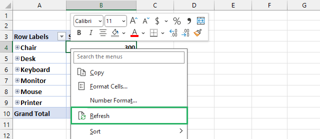
And it’s done! Your pivot table will be refreshed to show any updates in the dataset on the table.

Cool, no? 🤓

Refresh pivot table upon updating source data in Excel

If you change the pivot table data source, you will need to refresh it to reflect the new dataset.

That’s because a pivot table uses a pivot cache and the cache does not update automatically. Hence, to update the pivot table, you need to refresh the pivot cache to get the new data range 🤔

We will use the following dataset for the above-given pivot table. This will require updating the data range which is what we want to do in this example.

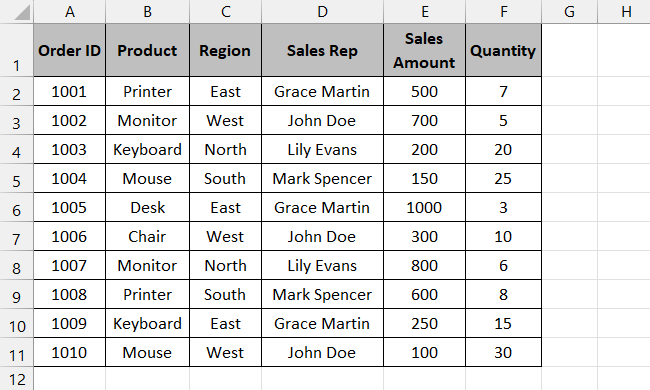
To change the data source,

Step 1) Click on the pivot table to activate it.

Step 2) Two new tabs will appear on the ribbon 🎀

Step 3) Choose the PivotTable Analyze tab and select Change Data Source from the Data section.

Step 4) If your pivot table is on a new sheet, Excel will take you to the original sheet containing the data set – if not it will show the Change Data Source dialog box on the same worksheet.

Step 5) From the table, select the new range of your dataset 💻

Step 6) Press Ok.

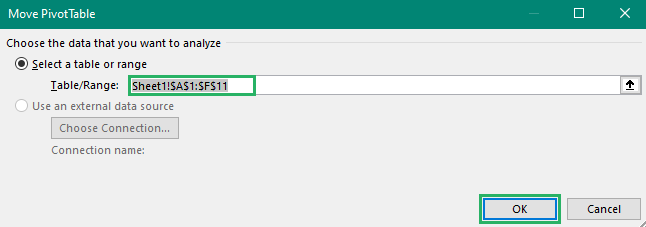
Your pivot table will be refreshed as:

How cool is that? 😃

Refresh multiple pivot tables

If you have more than two pivot tables in your dataset, using the simple Refresh technique will not update both tables simultaneously and updating each pivot table separately can be a hassle 😩

Luckily, we have a cool technique to refresh multiple pivot caches in one go in our workbook. We have the same pivot tables as earlier – only two more copies of it.

To refresh them together,

Step 1) Open the workbook.

Step 2) Go to the Data tab and click the Refresh All button from the Queries and Connections section.

And it’s done! Both the pivot tables in your workbook will be refreshed 🔃

Pro tip

There’s also a shortcut key to this method. Press Alt + A + R + A on your keyboard to use the Refresh All command. This is very handy if you prefer keyboard shortcuts.

Refresh the pivot table automatically as the workbook opens in Excel

If you have to work with the same pivot table frequently and want to automate the refreshing task, this method is for you. It automatically refreshes the pivot table as you open the workbook 📖

We have the same pivot table as earlier. Let’s see how you can automate refreshing your table.

To do that,

Step 1) Go to the PivotTable Analyze tab and click on Options from the PivotTable section.

Step 2) Go to the Data tab.

Step 3) Under PivotTable Data, check the ‘Refresh data when opening the file’ option.

Step 4) Press Ok 🆗

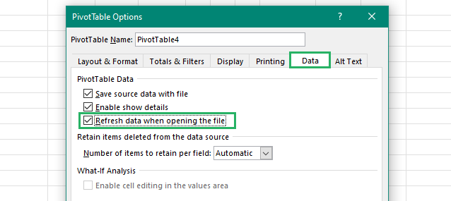
And it’s done! Now your pivot table will be refreshed each time you open your workbook.

Refresh the pivot table after a set period in Excel

You can also set automate your pivot table to refresh after every certain period. But you can only do this if your table is OLAP based 🤔

Let’s now see how to set the timer for refreshing the table.

Step 1) Go to the Data tab on the Ribbon and click on Properties from the Queries & Connections section.

Step 2) The Connection Properties dialogue box will appear on the screen.

Step 3) The User tab is selected by default.

Step 4) Check the Refresh every minute box to enable it.

Step 5) Now select the time you want the pivot table to refresh after – we set it to 10 minutes.

Step 6) Press Ok.

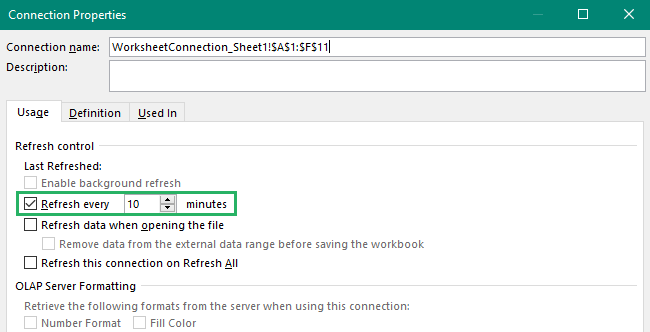
Voila! The pivot table will now refresh after every ten minutes – how cool is that? 😀

Refresh pivot table using VBA in Excel

Another cool method to refresh your Excel pivot table is to use VBA. This is a rather advanced method and is not recommended for beginners 😵

Our pivot table initially looks like this:

To refresh the pivot table using VBA,

Step 1) Press Alt + F11 on your keyboard ⌨

Step 2) Go to the Insert tab and click on Module from the dropdown.

Step 3) Paste the following VBA code into the window.

Step 4) Close the Visual Basic editor.

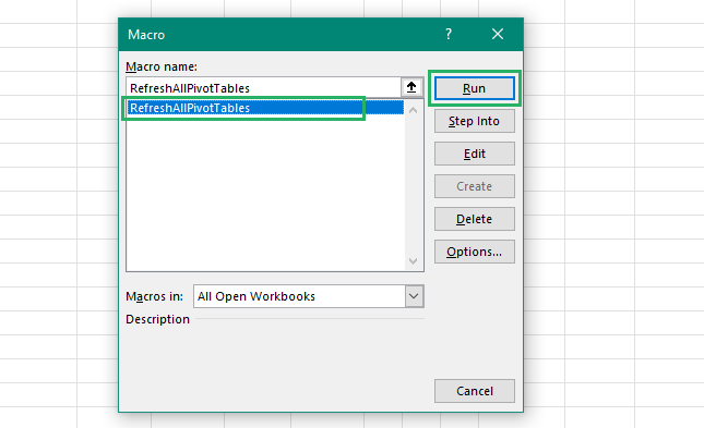
Step 5) Press Alt + F8 to run macros.

Step 6) Select the RefreshAllPivotTables macro.

Step 7) Press Run 🏃‍♀️

The Pivot table will refresh as:

How easy is that? 🧐

Conclusion

In this tutorial, we saw how to refresh pivot tables in Excel using different methods. We saw how to automate refreshing pivot tables, setting a timer and refreshing multiple tables at once.

We also saw how VBA can help us update pivot tables using macros and other simple methods like ribbon and right-click dropdown menu 📄

VBA is the prime method for experienced Excel users, whereas the right-click method is best suited to beginners. We also saw how you can stop a refresh process in the middle.

To learn more about pivot tables, check out our other pieces below.

How to Create a Pivot Table in Excel: Step-by-Step (2024)

How to Delete a Pivot Table in Excel – With and Without Data

How to Add Calculated Fields in Excel Pivot Tables (2024)

We hope you enjoyed reading this article as much as we did crafting it! 🤗