How to Add Calculated Fields in Excel Pivot Tables (2024)

Normally, you’d have to alter the source data to add a field to the pivot table. But with the calculated field, you can add a field to the pivot table without first adding it to the source data.

That creates an “imaginary” column where you can use your own formulas to grab data, or do calculations.

This is great for situations where editing the source data is impractical.

Let’s dive into how to add a calculated field to a pivot table 🤿

Download the sample workbook here if you want to tag along.

What are calculated fields

You can create calculated fields using formulas based on the existing fields of the Pivot Table.

The below example will help you to understand the Pivot table calculated fields.

The below Pivot table summarizes employee sales targets and sales actuals 💰

Now you need to find the sales achievement for each employee 🧑🏻‍💻

What happens if you calculate the sales achievement percentage outside the Pivot Table?

Then, calculations may not update with the Pivot Table updates.

There is a simple way to add a new calculated field to the Pivot Table as an Achievement percentage.

You don’t need to go and add a new calculation to your source data.

It is to add a calculated field to your Excel Pivot Table 🥳

How to add calculated fields

You can add a calculated field as an Achievement percentage to the pivot table by following the steps 🪜

1. Select any cell in the Pivot Table to activate the PivotTable Analyze tab and click that.

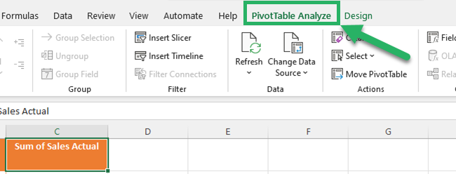
2. Expand the Fields, Items, & sets option in the Calculations group.

3. Click “Calculated Field…” to open the “Insert calculated field” dialog box.

4. Enter a name for the calculated field in the name box.

So, you can type “Achievement %” in the name box.

5. Enter the calculated field formula.

You can select a field and double-click or click the “Insert field” button to add the field to the formula box.

You can create your own calculated field formulas in this formula box.

In this case, you have to enter the following formula.

= ‘Sales Actual’/ ‘Sales Target’

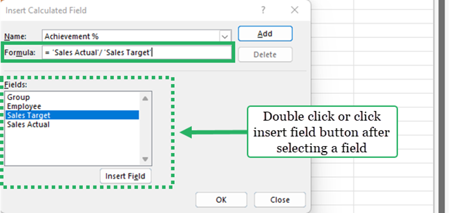
6. Click Add button or OK button to add the calculated field to the Excel pivot table.

You can see that the calculated field appears in the Pivot Table and the values area of the PivotTable fields box.

You can use the preferred number formatting for the calculated field.

Pro Tip:

Do you want to get all the formulas you have used for calculated fields in your Excel pivot table?

You have to follow the below steps.

1. Expand the Fields, Items, & sets option in the PivotTable Analyze tab.
2. Select the “List formulas”.

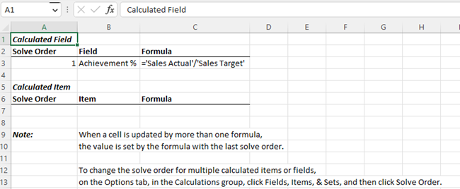
Excel displays all the details of calculated fields of the Excel Pivot Table in a new worksheet.

In this case, you can see the Pivot Table formula that you have used for the calculated field 🤩

You can modify or delete an existing calculated field if you need.

• To modify,

1. 1. Select the field name from Insert calculated field’s names list.
   2. Do the modifications in the name box and/or Formula box.
   3. Click the Modify button.

• To remove calculated fields;

1. 1. Select the field name from Insert calculated field’s names list.
   2. Click the delete button.

Disadvantages of calculated fields

Even though calculated fields are a very useful feature, it has some disadvantages ☹️

1. You can apply calculated fields only in regular Pivot Tables. If you have used data models for the Pivot table, calculated fields are not available for your Pivot table.
2. You cannot use name ranges or references when you are creating calculated fields. Due to that, you cannot use XLOOKUP, VLOOKUP, INDEX and functions that use references for calculated field formulas.
3. It may give wrong subtotals or grand totals for the Pivot table calculated fields. You can insert a new calculated field as commission to understand this point.

You can use the following formula to calculate the commission value based on total sales.

= IF(‘Achievement %’>100%,’Sales Actual’*10%,0)

You will get the below output.

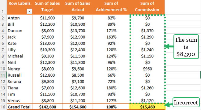
The grand total for the commission is calculated as actual total sales multiplied by 10%. It has not taken the total of the calculated items.

4. You cannot use calculated fields as a report filter or slicer.
5. The count of text fields cannot be used for the calculated field formula. If you use it, the result will be zero.

You can create a calculated field for the below Pivot table.

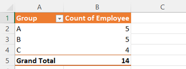
Assume that you want to multiply the count of employees in each group by the $1,000 allowance to calculate values for allowance.

You can use the below formula for that.

=Employee *1000

Your output will be as follows.

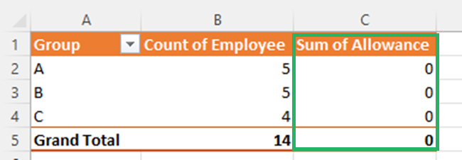
All the calculated values are zero 0️⃣

This is because the calculated field is not using the count of employees of the Pivot Table field.

It is using the data fields in the source data. Those text fields do not have any numeric value and the value is zero.

That’s it – Now what?

Now you know how to quickly create a calculated field for a pivot table. Well done!👏🏻

Have you noticed that when you are entering the formula for the calculated field, it will not show the arguments for the functions? 🤔

Therefore, it is vital to be thorough with functions such as IF, SUMIF, and VLOOKUP.

To master these functions, all you need to do is enroll in my free 30-minute online course.

Other resources

If you want to learn more about Pivot tables, read our article about Pivot Tables.

You can insert calculated fields in the Pivot Tables of your dashboards.

If you are interested to know how to make a dashboard in Excel, read this tutorial. Or check out my top-6 dashboard templates here!