How to Remove Duplicate Rows in Excel (The Right Way)
Working with large datasets in Excel often involves dealing with duplicate rows which can be a tiresome task to eliminate.
To maintain data quality in your spreadsheet, you need to remove all duplicate values whether you are storing customer records or tracking inventory 🤔
Luckily, Excel offers a variety of ways you can use to clean data in your worksheet. In this tutorial, we will see different ways you can use to remove duplicate rows in no time.
Download our sample workbook below so you can practice alongside the guide 📖
Remove duplicates using the built-in Excel feature
The easiest and most common method of removing duplicates in Excel is to use the built-in Remove Duplicates feature. It scans a dataset and removes duplicate data.
Say, we have the following data set containing multiple duplicate entries. We want to remove duplicate values using the remove duplicates feature 📑
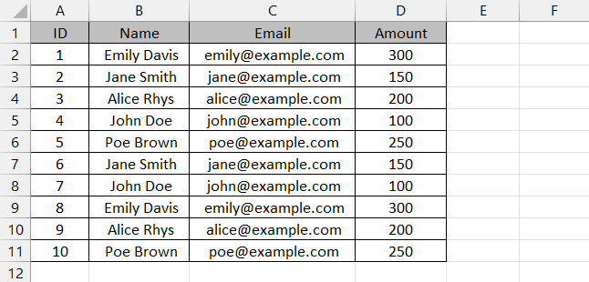
To do that,
Step 1) Select the range of cells containing your data.
Step 2) Go to the Data tab and select the Remove Duplicates option from the Data Tools section.

Step 3) The Remove Duplicates Dialog box will appear.
Step 4) If your dataset doesn’t have headers, untick the My data has headers box otherwise leave it be.
Step 5) All columns in your dataset are selected by default.
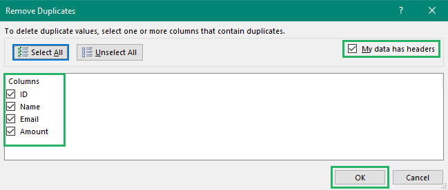
If you want to choose selective columns in your dataset, you can uncheck columns not needed. Or you can click the Unselect All option and then select the columns you want to remove duplicates from.
Step 6) Once done, press OK.
A Microsoft Excel dialog box will appear on the screen mentioning the number of duplicates and unique records found and removed. Click OK and it’s done! 😃

The duplicate values in your dataset have been removed. How cool is that?
Remove duplicates using an advanced filter
The Advanced Filter feature in Excel offers an easy way to remove duplicate values. It filters out the duplicate records and copies the unique values to a new column.
To use an advanced filter,
Step 1) Go to the Data tab and click on Advanced from the Sort & Filter section.

Step 2) The Advanced Filter dialog box will appear on the screen 💻
Step 3) Select the action you want to perform, whether you want to filter the values in place or copy to a new location – we will filter in place.
Step 4) Select the range containing duplicate values in your Excel spreadsheet.
Step 5) Check the Unique Record only box at the bottom.
Step 6) Press Ok.
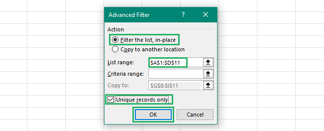
The duplicate values will be filtered to retain unique values as:

Pretty cool, right? You can also copy these values to a different location 🚩
Remove duplicates using conditional formatting
Another convenient way of removing duplicates from your data set is to use conditional formatting. It requires applying a rule to your data set and the values that match the rule are eliminated ❌
We will use the same dataset as earlier where we want to filter out the duplicate values.
To do that,
Step 1) Select the dataset containing the duplicate values.
Step 2) Go to the Home tab and select the Conditional Formatting button from the Styles section,
Step 3) From the dropdown that appears select Highlight Cell rules.
Step 4) Click on Duplicate Values at the end of the dropdown list.
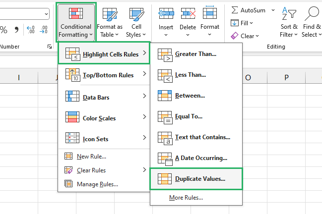
Step 5) The duplicate values dialog box will appear on the screen.
Step 6) Select the type of value you want to color – unique or duplicate.
Step 7) Select the color you want to format the cells meeting the condition.
Step 8) Press Ok.
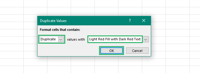
All the cells containing unique values will be formatted as:
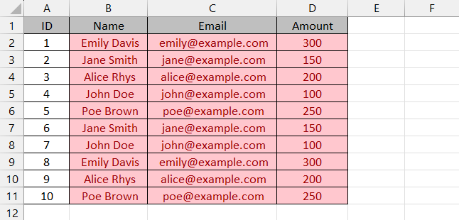
You can now remove the duplicate values using the advanced filter as seen above to get unique values as:

Remove duplicates using Pivot Table
A pivot table is another fun way of removing duplicate entries in Excel. It makes you an entire table of your data set only without the duplicate values 🧐
To do that,
Step 1) Select all of your dataset.
Step 2) Go to the Insert tab and click on Pivot Table in the Tables section.

Step 3) The Pivot Table dialog box will appear on the screen.
Step 4) Select the New worksheet option and press Ok 👍
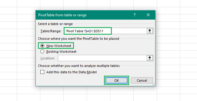
Step 5) A new empty pivot table will appear on a new worksheet on the left side.
Step 6) On the right, there will be a Pivot pane.
Step 7) Select column names from the fields and add them to the Rows area in the following order:
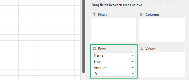
Step 8) Once done, go to the Design tab on the ribbon and click on the Report Layout button from the Layout section.
Step 9) Select Show in Tabular Form from the dropdown list.
Step 10) Now, select the Grand Totals and Subtotals options and turn them off.

This is what the final pivot table will look like after adjusting the column width:
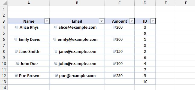
How cool is that? 🤓
Remove duplicates using Excel formulas
You can also use Excel formulas to remove duplicate rows in your data set. This method can be slightly more time-consuming but it works pretty neat for large Excel sheets 📗
We are going to use the IF and COUNTIF function in this example. The syntaxes of the two are given respectively:
where,
logical_text refers to the condition to be tested
value_if_true refers to the value to print if the function returns true.
value_if_false refers to the value to be printed if the function returns false
and,
where,
range refers to the range containing values you want to count
criteria refers to the condition to be tested against the range of cells
We will use the same sample data as earlier. We want to filter out the rows containing duplicate values by using the above two formulas using a helper column. We will then filter out the duplicate values using that column.
To do that,
Step 1) Select cell E1.
Step 2) Type in your column header – in our case Dupes.
Step 3) In cell E2, type in the following formula.
The formula counts the number of times the text in B2 (criteria parameter) appears in the entered range. If the text appears more than once, it prints “Duplicate” in the helper column, otherwise it prints “Unique”. The criteria reference adjusts according to the current cell the formula is dealing with.
Step 4) Double-click the Fill Handle at the bottom right corner of the active cell to copy the formula down to the remaining cells.
The final result will look something like this:
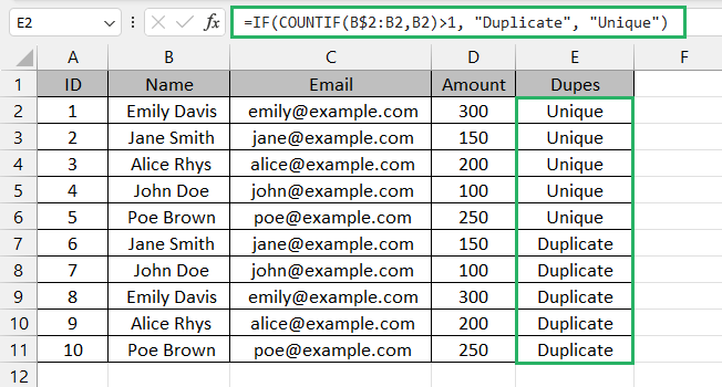
Once you have the helper column, now’s the time to filter out our unique values.
Sep 5) Right-click Dupes or the helper column.
Step 6) From the dropdown list that appears, click on Filter 🦯
Step 7) Select Filter by Selected Cell’s Value.
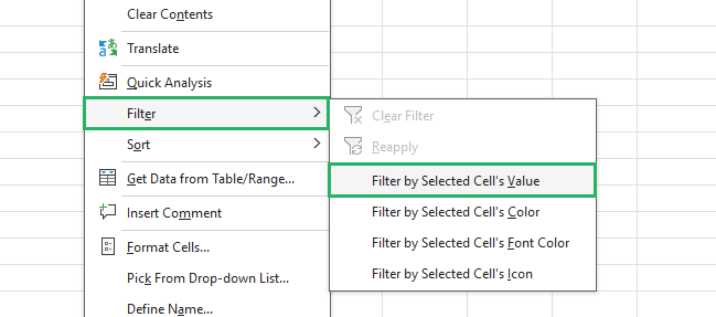
Step 8) All values will disappear from your dataset.
Step 9) Now, click on the little funnel icon at the right corner of your column header.
Step 10) Select Unique under the Select All checkbox.
Step 11) Press Ok.
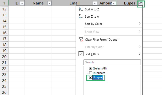
And it’s done! 🥇
The filter will display only the unique values in your dataset while hiding the duplicate values:

The best part is your original data also remains intact. How cool is this method? Try it now!
Remove duplicates using VBA
An advanced but quick method of removing duplicates in Excel is to use VBA. For this example, we will be running a simple macro.
To do that,
Step 1) Press Alt + F11 on your keyboard ⌨
Step 2) The Visual Basic editor will open on the screen.
Step 3) Go to the Insert tab and select Module from the dropdown list.

Step 4) Paste the following code in the Module window.
Step 5) Now close the editor.
Step 6) Press Alt + F8 to open the Macros window.
Step 7) Select RemoveDuplicates and click Run 🏃♀️
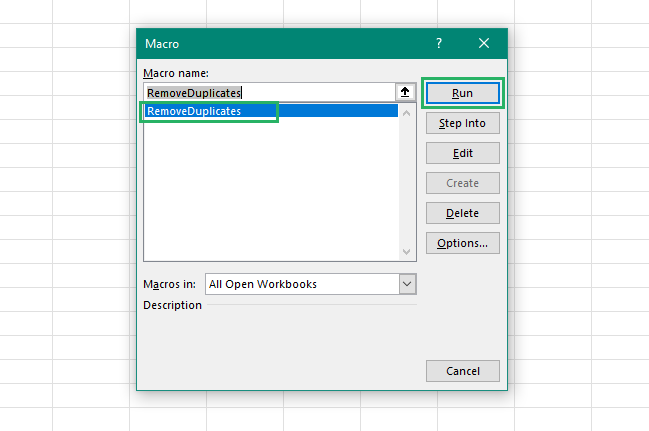
All the duplicate values in your dataset will be removed with only unique values remaining as:

Pretty cool, no? 🧐
Conclusion
In this guide, we saw how to remove duplicate rows using Excel’s built-in feature, conditional formatting, and pivot table. We also used some advanced methods like Excel formulas and VBA.
You can use any method you like but for a beginner, we would suggest using Excel’s removing duplicate feature or advanced filter 🔍
To learn more about conditional formatting and pivot tables in Excel, read these articles below.
How to Create a Pivot Table in Excel: Step-by-Step (2024)
How to Sort a Pivot Table in Excel: Step-by-Step (2024)
How to Use Conditional Formatting to Highlight Text in Excel
We hope you enjoyed reading this article as much as we did crafting it! 🤗
