How to Sort a Pivot Table in Excel: Step-by-Step (2024)

When you deal with large amounts of data in your Pivot table, knowing how to sort data in it is really helpful 😀

Excel offers you a lot of sorting options for you to easily sort data in your Pivot Tables. And with a sorted pivot table, you can find and analyze the presented data quickly 📈

In this lesson, you will learn how to sort a pivot table by Pivot table values, by text, and by custom order in Excel.

Download the attached Excel workbook to practice this lesson, and let’s start 💪

Table of Contents

Sort a pivot table by values
Sort a pivot table by text (from A-Z)
Custom pivot table sorting
That’s it – Now what?

Sort a pivot table by values

The below Pivot Table shows the sales data of a hotel. The column labels show the day of the week. The row labels show the package.

You can sort the values of the above pivot table, vertically as well as horizontally ⬆️➡️

Sort pivot table vertically

Assume that you want to get the highest sales contributing package to the top of the list.

Then, you have to sort the Pivot Table vertically in descending order.

Follow the below steps to sort Pivot Table data.

Click the small drop-down arrow in row labels.

Click the small drop down arrow in row labels in the Pivot Table.

Select more sort options from the drop-down list.

Select more sort options from the drop down list

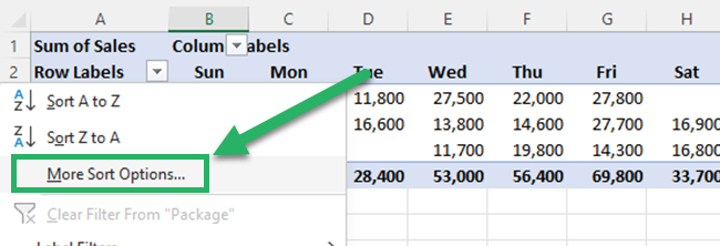
To sort descending order select “Descending (Z to A) by:”.

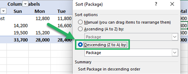
Select descending order from sort options.

Click the down arrow button below that and select the sum of sales column.

Click the down arrow below that and select the sum of sales column.

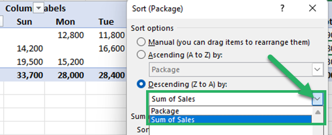
Click the “OK” button to sort data.

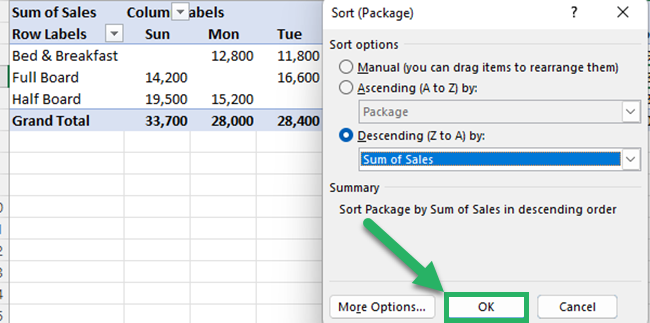
Then, packages will be sorted based on the value field.

Sort pivot table horizontally

Imagine that you want to sort pivot table days based on sales value. You can arrange it from the smallest value to the highest value.

So, you must sort the Pivot Table horizontally in ascending order.

You can follow the below steps for that.

Select any value in the Pivot table’s grand total row except the cell in the grand total column. So, you can select any cell in the range of B6 to H6.

Select any value in the Pivot table's grand total row except the cell in the grand total column

Go to the Data tab.

Click the custom sort icon of the sort and filter group in the data tab.

Then the sort-by-value dialog box appears. To sort in ascending order, you have to select smallest to largest from the sort options dialog box. Select the largest to the smallest sorting option, if you want to sort data in ascending order.

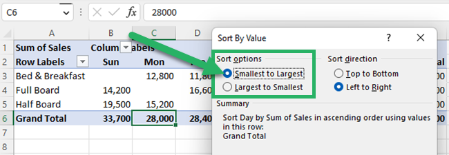
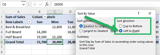
Select left to right as the sort direction as you want to sort horizontally.

Click OK.

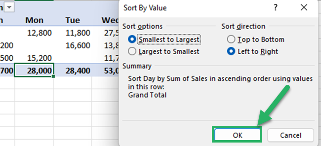
Your Pivot Table is sorted horizontally in ascending order.

Sort a pivot table by text (from A-Z)

In Pivot Tables, you can sort text as well. A Pivot table field that contains text can be sorted in alphabetical order.

You cannot sort Pivot Tables by following ⛔

Case-sensitive text entries

Conditional formatting indicators/ icon sets

Cell color

Font color

Kasper Langmann, Microsoft Office Specialist

The packages in below Pivot Table are not in alphabetical order.

A Pivot table to sort alphabetical order

If you want to arrange packages in alphabetical order, you can follow the below steps.

Right-click on any cell that contains a package name. So you can select any Row label in cells A3 to A5.

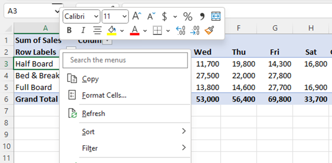
Go to the “sort” option in the menu.

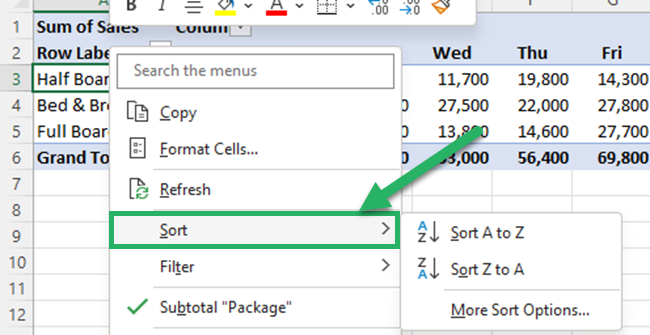
Select “Sort A to Z” to sort in alphabetical order.

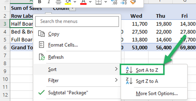
Now the Packages are sorted in alphabetical order as follows.

Pro Tip:

If there are leading spaces, it will distort PivotTable data sorting 😫

So, before you sort text items, make sure to remove leading spaces.

Custom pivot table sorting

Pivot Table sort options are not limited to numeric values or alphabetical order 🤔

You can sort Pivot Table based on a custom order or own custom lists 🥳

In the below Pivot Table, days are not sorted alphabetically order.

Days of the Pivot Table are sorted alphabetical order.

If you want to sort days as per the order of the days of the week, you have to do the following.

Select any cell in the days row.

So, you can select any cell in the range of B2 to H2.

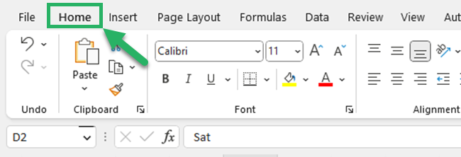
Go to the Home Tab.

Click the sort and filter button in the editing group.

Click sort and filter button in the editing group

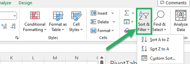
Select custom sort options.

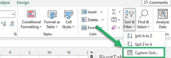
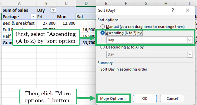
Select the “Ascending (A to Z) by” sort option and click the “More options…” button.

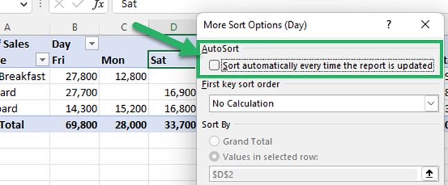
Uncheck the automatic sorting option. Then, your table will not sort automatically.

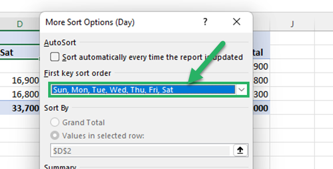
Expand the drop-down list of “First key sort order” to see the inbuilt custom lists.

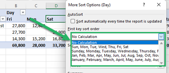
Select “Sun, Mon, Tue, …” as the custom list and click “OK” twice.

Now your Pivot Table will sort as below 😍

Pro Tip:

Sometimes you add new items to the source table.

Those new items are coming at the end of the Pivot table’s report filter.

Even a manual sort is not possible for report filters.

The solution is to move the report filter to rows or columns and apply the Excel sort option in the same way you did earlier.

Then move that Pivot item again to the report filter area 🤗

That’s it – Now what?

Well done! 👏🏻 Now you know all the methods to sort a pivot table field. Whether it’s by values, by text, or by your own custom list.

Excel makes sorting data in Pivot tables so easy! With a few clicks, you can find and analyze the data in your Pivot tables.

If you want to do a lot of tasks with just a single click of your mouse, then it’s time for you to know more about Excel macros. You can automate your workflow (and a whole lot more) using Excel macros 🤯

Join my Excel Advanced user training where you’ll learn the basics of Excel Macros with me.

Other resources

If you want to learn everything you need to know about sorting data in Excel, don’t forget to read our How to Sort in Excel: Data and Columns guide.

Dive deep into Pivot tables and how to create them 🤿

You can apply all your Pivot Table skills to create amazing dashboards in Excel (+free templates here).