How to do Sensitivity Analysis in Excel (Easily)
Excel is a great analytical tool and if you haven’t yet used it for sensitivity analysis, you’re missing out on a great feature of Microsoft Excel.
The sensitivity analysis tool of Excel allows you to see how variation in one or more input variables may impact the output of the model.
You can systematically list down a range of input variables and try them all to see how sensitive the output to this input variation is. Helps you identify the critical factors so you can make informed decisions.
Projecting it to the world of finance, sensitivity analysis has a broad scope of application. In this guide, I will take you through two methods to do sensitivity analysis in Excel like a breeze.
Grab your free practice workbook for this guide now and tag along with me.
What is Sensitivity Analysis
Whenever you’re budgeting or forecasting data under a model, you are taking a handful (or more) of assumptions and relying on their outcome.
Since these are just your expectations that might go unrealistically well or horribly wrong – you can only hope and project but never be sure about them. That is where and why you perform a sensitivity analysis (also called stress testing).
We stress some of the critical assumptions of our data model to see how worse the results can get with different scales of changes to our assumptions. This is to see the results your financial model would yield under different circumstances.
Sensitivity analysis is all about analyzing how sensitive are results of your data model are to different variable inputs.
We are going to cover two comprehensive examples of performing sensitivity analysis in Excel just now. Let’s jump down straight to understand it better.
One variable sensitivity analysis in Excel
To understand how single variable sensitivity analysis is performed in Excel, let me show you this example. I have $10,000 that I want to invest for 5 years.
Different instruments and banks offer different interest rates. I want to see what the final lump sum amount that I will draw from the instrument after 5 years (principal and interest included).
Here’s how we do it.
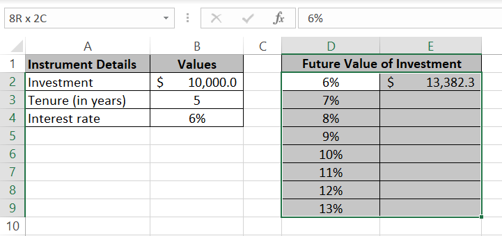
For an exemplary interest rate of 6%, the future value of my investment would grow to $13,382.
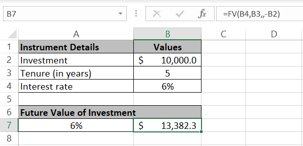
I have used the FV function of Excel to calculate the future value of my investment given the tenure of investment and the interest rate of 6%.
Now to see how different would be the future value of my investment under different interest rates, I am running a sensitivity analysis through the following steps.
Step 1) Make a two-column table (we call it a one variable data table).
Step 2) In the first column, populate the different interest rates for which you want to calculate the future value.
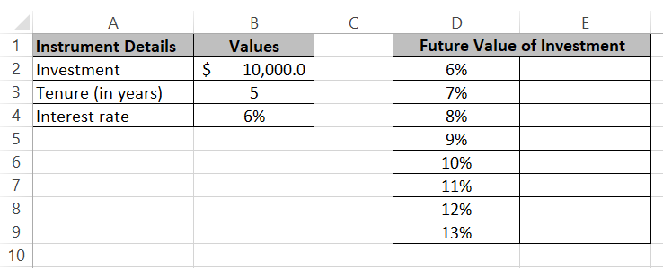
Step 3) In the first row of this table, write the exemplary interest rate i.e., 6%.
Step 4) In the column next to it, calculate the future value of your investment using 6% as the interest rate and reference all arguments from the original data table.
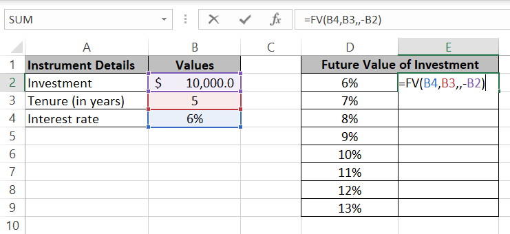
Step 5) This will calculate the future value for this investment at 6% in the first row of the table.
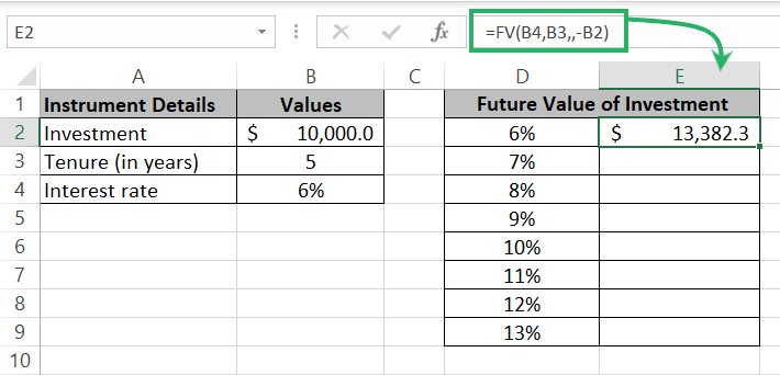
Step 6) Now select the entire range including the first row where we have already calculated the investment’s FV.
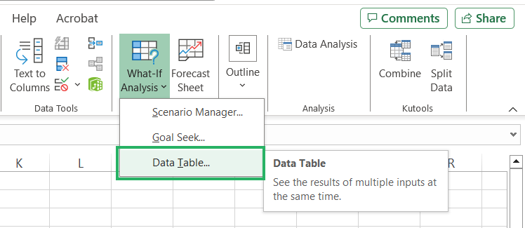
Step 7) Go to the Data tab > Forecast group > What-if Analysis > Data Table.
Step 8) From the Data Table dialog box that opens up next, refer to the interest rate (6%) from the original data table as the Column Input Value.
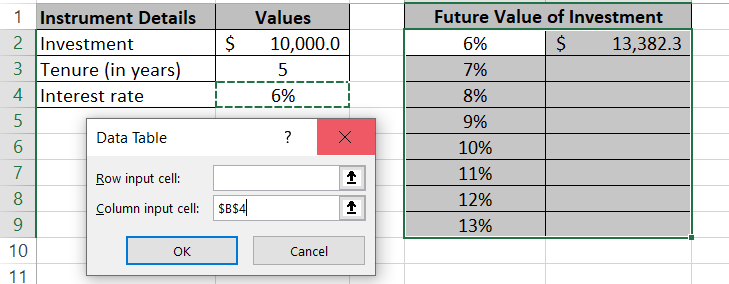
We have a column of interest rates that we want to be populated with the investment’s future value, so we have chosen Column Input Value and not Row Input Value. Plus, our dependent variable is the interest rate, so we have referred to it as the input value.
Step 9) Click on Okay.
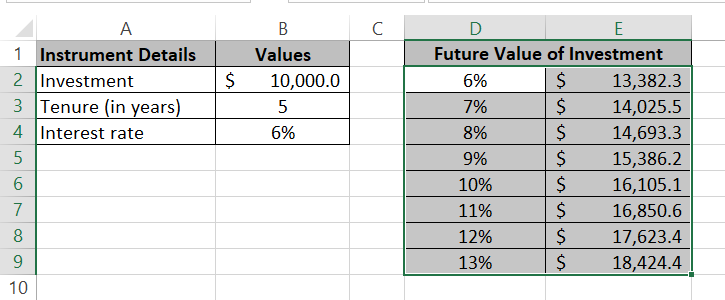
The Data table will calculate the future investment value for each of the interest rates in the first column using the same input values and formula as has been used to calculate the FV in the first row of the table.
This shows how sensitive is the future value of my investment to the interest rate. Increasing the interest rate by each one percentage leads to how much change in the FV of investment.
This is how you can instantly see how changes in input variables will affect the final results of any data model. Hope you found it interesting.
Two variables sensitivity analysis in Excel
If you liked doing a single-variable sensitivity analysis above, you’ll love the two-variable sensitivity analysis that you can perform in Excel.
In this example, I have a short Profit & Loss statement for my business. This is calculated using a set level of quantity sold and price per unit which is 1000 units sold at the rate of $50 per unit.

This yields me a net profit of $25,000.
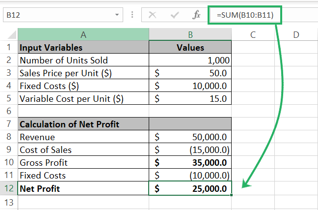
To see how I can better optimize my business, I want to see the net profit my business makes at different volumes and prices of sold units.
We will again leverage the What-If Analysis tool of Excel to see how sensitive my business to the volume and price levels of the units is sold.
Step 1) Create a two-dimensional table with different volumes on one side (within a column) and different prices on the other side (as a row).
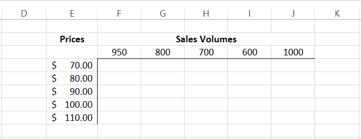
Step 2) In the first cell of the two-dimensional table, write in the same formula as used in the P&L statement to calculate the net profit for the volume and price in the original dataset i.e., for 1000 units and price of $50 per unit.

This formula is simple the price per unit multiplied by the units sold less the cost per unit multiplied by the units sold and then finally less the fixed costs.
Make sure to refer to cells from the original data table.
Step 3) Select this entire range (two-dimensional table) including the first cell with the pre-defined volume and price.
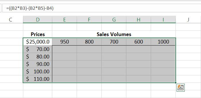
Step 4) Go to the Data tab > Forecast Group > What-if Analysis > Data Table.

Step 5) As the Row Input Value, refer to the Volume from the original data table as we have written different volume levels within the row.
Step 6) As the Column Input Value, refer to the Price from the original data table as we have written different price levels within the column.
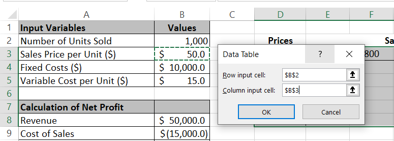
Step 7) Press Okay to have the net profit calculated for each combination of price and units’ level within the matrix.
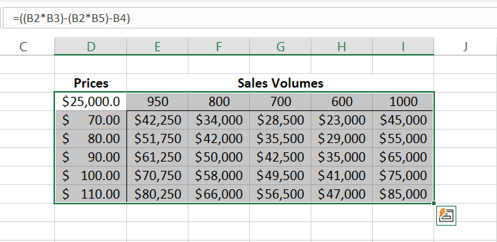
Wufh! This is insane.
Had you tried doing the manually (calculating the revenue and cost of sales and then the net profit) for like so many combinations of volume and price levels, it would have taken you hours to populate this table?
And let alone the chances of manual errors with such voluminous calculations. Populating them all together in a table would have been another task.
So, speaking of the What-if Analysis tool of Excel, it simplified the job for us multiplefold. It’s about pulling together different levels of inputs. setting up a formula, designating the input variables, and then clicking the Okay button.
Excel handles the rest.
Conclusion
In this guide, we have unveiled how to use sensitivity analysis in of Excel.
It helps you understand the dynamics of your data model and the influence of each input variable on the output. Leveraging the sensitivity analysis tool of Excel, you can not only understand the critical elements of your dataset, but you can make informed decisions that are resilient to change.
- Practicing the one-variable and two-variable examples explained above, you can easily master sensitivity analysis in Excel. And after you’ve done that, make sure to check out the following Excel tutorials by Spreadsheeto.
- Quick Analysis Tool in Excel: Full Tutorial (2024)
- How to Add the Data Analysis Toolpak in Excel (2024)
- How to Add Line of Best Fit in Excel (Easy Method)
