How to Sort Multiple Columns in Excel (Many Examples)

Have a tightly packed dataset that’s all out of order?

Don’t waste time sorting it manually and end up making mistakes that might ruin the accuracy and precision of your data.

Instead, let Excel wear the data-sorting cap for you. In this tutorial, we will see how you can sort multiple columns in Excel in one go.

And take it from me, you’ll be amazed to see how this works. So, let’s not waste any more time.

Get your free practice workbook for this guide here, and come along with me.

Table of Contents

Simple Sorting in Excel

Simple sorts (based on smallest to largest numbers) or A to Z (or vice versa Z to A) in Excel are pretty simple.

Excel can interpret huge sets of data and can sort them in any order as long as it’s based on a single column.

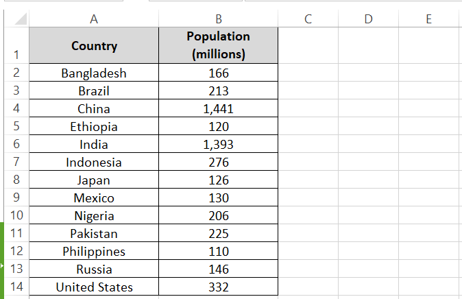
For example, I have a country-wise population in Excel.

To sort this data based on population size, say largest to smallest, follow these steps:

Step 1) Select the population size

Step 2) Go to the Home Tab > Editing group > Sort & Filter.

Step 3) Select Largest to smallest from the drop-down sorting menu.

You will see a Sort Warning next that asks if you want to expand the sorting to the adjacent columns as well (the country names).

Step 4) Choose the option to expand the selection.

Step 5) Click Ok.

The data will be sorted in the order of population size (largest to smallest).

Similarly, you can sort this data by arranging the countries in alphabetical order. To do so:

Step 1) Select the column containing country names.

Step 2) Go to the Home tab > Editing group > Sort & Filter > Sort A to Z.

Step 3) From the Sort warning, again choose to expand it to the selection.

The data will be sorted with the countries arranged in an alphabetical order (A to Z).

This is how simple sorting in Excel works where we sort a column, and the remaining data is accordingly arranged.

Sort Multiple Columns in Excel

As simple as simple sorting in Excel is, sorting your data by multiple columns is not difficult either.

Let’s see this through the following example.

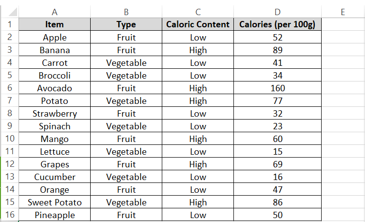
I have a set of data in Excel that mentions some food items, their classification, caloric classification, and then calorie content.

I want to sort it out to make out my diet plan. But since I am more of a Fruit lover, I want the sorting to be done in three steps as below:

• Fruits on top
• Within fruits, low-caloric fruits
• Within low-caloric fruits, fruits with the least to most calories

Sounds doable. Here we go sorting data.

Step 1) Select any cell from the data.

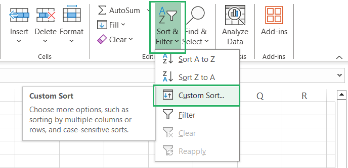
Step 2) Go to the Home tab > Editing group > Sort & Filter > Custom Sort.

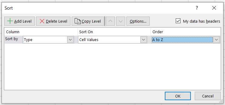
This will launch the Sort dialog box as this.

Step 3) Click on the Add Level button.

This will add a sorting level to it.

Step 4) Within this sorting level, under Sort By, select the first sort level, which is Type.

Step 5) Set “Sort On” to Cell values.

Step 6) As we want Fruits on top which starts with F, and the Vegetables next which starts with V, sorting data in A-to-Z order should do.

Cool! The first sorting level is defined.

Step 7) Again, click on the Add Level button to add the “Then By” Sorting level.

Step 8) Within this sorting level, under Sort By, select the second sort level, which is Caloric Content.

Step 9) Set “Sort On” to Cell values.

Step 10) As we want Low on top, which starts with L, and High, which starts with H, sorting data in Z-to-A order should do.

Now, for the third and last sorting level:

Step 11) Add another sorting level by clicking on the Add Level button.

Step 12) Within this sorting level, under Sort By, select the third sort level, which is Calories.

Step 13) Set “Sort On” to Cell values.

Step 14) As we want the calories to be arranged from lowest to highest, set the Order to Smallest to Largest.

Step 15) Click the okay button, and here’s what you get.

Wow! All my meal preferences are sorted in a jiffy. This is amazing.

The Sort tool of Excel makes multiple-level sorting in Excel super easy and automated. Hope this explains how you can sort multiple columns in Excel.

Sort Multiple Columns in Custom Order

Another interesting way how you can sort data in Excel is by defining the custom sorting order yourself.

How? Check this example out.

Here’s my inter-company data on the employees’ performance from different departments.

Now if I want to know which employees performed the best to worst in each department, it will take me quite some time to sort those details out since the data is all jumbled up.

I need to sort it out in two levels:

• Employees from Marketing, Sales, HR, and IT arranged in order
• In each department, ranking employees in the order of best performance i.e., Excellent, Good, Satisfactory, and then Poor.

To sort this data in this order, follow these steps.

Step 1) Select any cell from the data.

Step 2) Go to the Home tab > Editing group > Sort & Filter > Custom Sort.

Step 3) In the Sort Dialog box, click on the Add Level button to add a sorting level.

Step 4) Within this sorting level, under Sort By, select the first sort level, which is Department.

Step 5) Set “Sort On” to Cell values.

For Order, note that Excel only offers two pre-defined orders to sort values (A-to-Z and Z-to-A).

However, none of these predefined orders suit us. Our desired order of Marketing, Sales, HR, and IT is [M, S, H, I].

This is an alphabetically jumbled order. To arrange the data in this order of departments, a custom order list needs to be set up.

Here’s how you do it.

Step 6) For the Order, select Custom List.

This will launch the Custom List dialog box as follows:

It already has some pre-defined custom lists for the days of the week.

Step 7) Click on New List to define a list of your own.

Step 8) In the List entries box, type the department names in the desired order with a line break after each department.

Step 9) Click on the Add button to add this list of entries to the pre-defined lists.

Step 10) Select this list and press okay.

This takes us back to the Sort Dialog box, where we will now define the second level of sorting.

Step 11) In the Sort Dialog box, click on the Add Level button to add a sorting level.

Step 12) Within this sorting level, under Sort By, select the second sort level, which is Performance.

Step 13) Set “Sort On” to Cell values.

We again do not have a preset order to input. We want the performances to be graded from the worst to the best, which makes the order Excellent, Good, Satisfactory, and Poor [E, G, S, P].

Talking of alphabetical order, this is neither a perfect A-to-Z nor a perfect Z-to-A. Hence, no chance of relying on predefined orders.

We will have to customize the order ourselves.

No worries! Let’s do it.

Step 14) For the Order, select Custom List.

Step 15) In the Custom List dialog box, select the option for a New list.

Step 16) In the List entries box, type the performance grades in the desired order with a line break after each grade.

Step 17) Click the Add button and then the Okay button.

This is how the Sort dialog box finally looks.

Step 18) Press okay again.

And there you go! Excel sorts the data based on the Custom lists defined by you.

We have all the employees from the Marketing, Sales, HR, and IT grouped in order. And then within each department employees are arranged based on best to worst performance.

Interesting! The Custom List feature of the Sort & Filter tool takes a minute to clean and organize data.

This is how you can sort multiple columns in Excel based on custom listings.

Conclusion

The Sort & Filter tool of Microsoft Excel is amazing. Especially sorting data on multiple levels (up to 64) based on different criteria is somewhat mind-blowing.

All in all, this is one tool to sort data in Excel. In addition to it, there’s so much more that you can do in Excel to sort your data amazingly quickly.

Check these out by reading our following Excel tutorials on sorting data.

• How to Sort a Pivot Table in Excel: Step-by-Step (2024)
• Excel SORT Function: Sort Excel Data Using a Formula (2024)
• How to Sort Columns in Excel (Without Mixing Data)