How to Sort Numbers in Excel (Lowest to Highest, etc.)
Microsoft Excel allows you not only to store data in your worksheet but also to organize them.
One of many ways to organize your data is by sorting them. You can sort data by specifying criteria such as cell values, cell color, font color, or conditional formatting icon. 🔍
In this tutorial, we’ll focus on how to sort numbers in Excel. Whether you need to sort numbers in a single column or multiple columns, we’ve got you covered. 😃
Download this sample workbook and let’s sort!
Sort Numbers in Excel – Single column
Sorting numbers in Excel is as easy as 123.
You can rearrange numbers in a single column from lowest to highest, or vice versa.
Open your sample workbook and you’ll find numbers arranged randomly.
Lowest to Highest
To sort these numbers from Lowest to Highest, you need to:
Step 1) Select the data you want to sort.
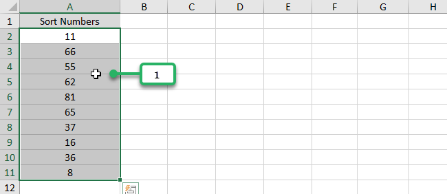
Step 2) Go to the Data Tab.
Step 3) In the Sort & Filter group, click the A to Z command. This quickly sorts data from smallest to largest or in ascending order.

Easy as 123, right? 😉
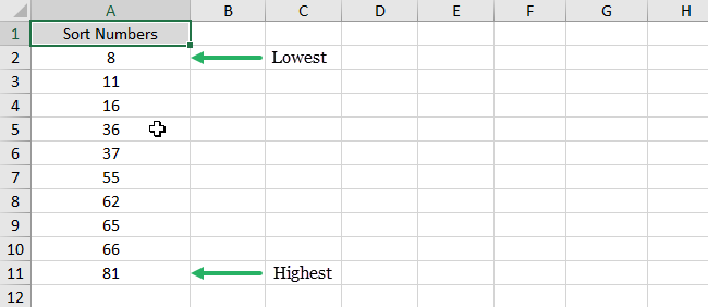
Highest to Lowest
In the same way, to sort numbers from Highest to Lowest,
Step 1) Select the data you want to sort.
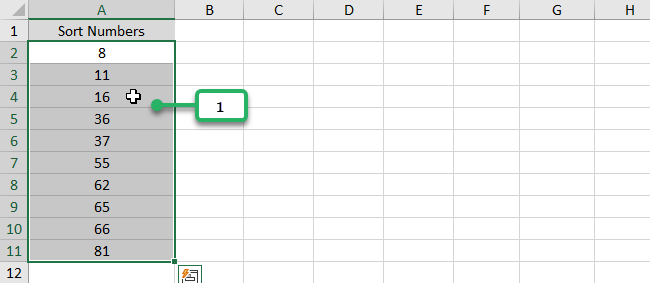
Step 2) Go to the Data Tab.
Step 3) In the Sort & Filter group, click the Z to A command. This quickly sorts data from largest to smallest or in descending order.

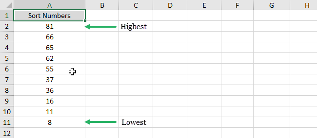
Sort Numbers in Excel – Multiple columns
In the real world, we just don’t sort data in single columns. We work on Excel worksheets with columns and columns of information and need to sort data in multiple criteria.
It could be sorting employees’ names in the department in alphabetical order, then sorting numbers by highest sales for reports. 📊
Learning how to sort numbers in multiple columns is important as it allows you to find values quickly in your worksheet.
It’s not as easy as 123, but you can do it! 💪
In our sample workbook, you’ll see 3 columns. Column A shows you the department where the employees belong (Column B) and their Annual Salary in Column C.
Let’s try to sort numbers and arrange the data from highest to lowest in terms of Annual Salary.
However, when sorting numbers in multiple columns, you can’t simply click the A to Z or Z to A commands.
Let’s follow these steps:
Step 1) Select the data range you want to sort.
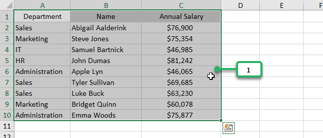
Step 2) Go to the Data Tab.
Step 3) In the Sort & Filter group, click the Sort command. This will open the Sort dialog box.

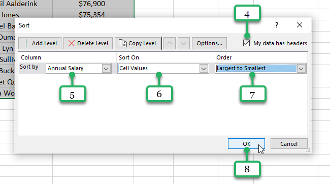
Step 4) Since our Excel table has a header (first row), tick the “My Data has headers” checkbox on the top right corner of the Sort dialog box. If this box is not ticked, your header will be treated as data.
Step 5) Click on the “Sort by” dropdown list. This will show you the columns of your Excel table.
Select the “Annual Salary” column.
Step 6) Click on the “Sort on” dropdown list. This will show you the options you can choose from: “Cell Values”, “Cell Color”, “Font Color” and “Conditional Formatting Icon”
Select “Cell Values”.
Step 7) Click on the “Sort order” dropdown list. Since we’ve selected Cell Values, this will show you the options: “Smallest to Largest”, “Largest to Smallest”, and “Custom List”
Select “Largest to Smallest.”
Step 8) Finally, click OK.
This is now the result. 👍
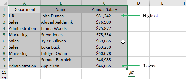
Our Excel table is now arranged from highest to lowest in terms of salary among all the employees.
This is an example of a single-level sort. However, in MS Excel, you can add more levels.
For example, let’s try to sort data by department first, and then sort by numeric values in terms of their Annual salary.
To do that, 👇
Step 1) Select the data range you want to sort.
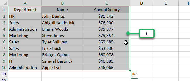
Step 2) Go to the Data Tab.
Step 3) In the Sort & Filter group, click the Sort command. This will open the Sort dialog box.
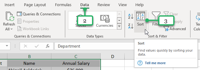
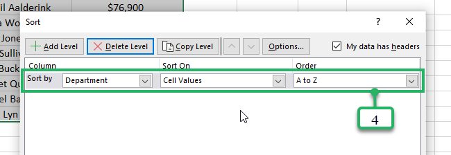
Step 4) First, let’s sort data by department following the criteria below.
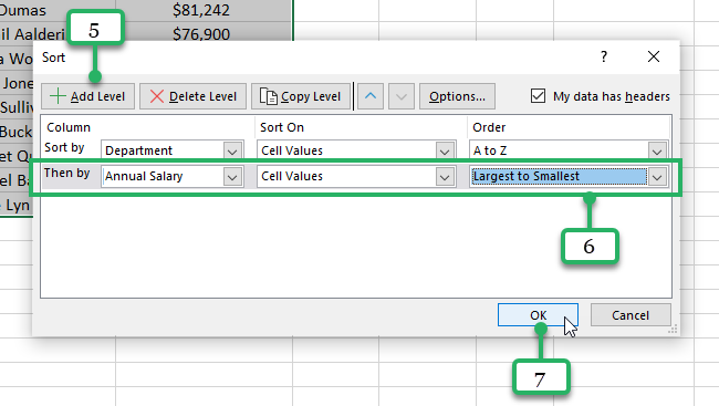
Step 5) To add another level, click “Add level” on the top left corner of your Sort dialog box.
Step 6) For the second level, sort numbers by Annual Salary following the criteria below.
Step 7) Finally, click OK.
Your Excel table now looks like this. 👀
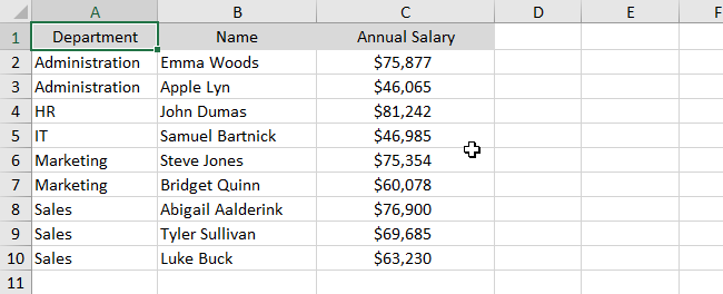
This is called multiple-level sorting. You can see each of the departments grouped, and employees’ salaries arranged from highest to lowest in their department.
That’s It—Now What?
Great work!
Today, you’ve learned how to sort numbers in Excel, not only in single columns but also in multiple columns and on multiple levels. It’s a quick way to organize your data and find the important values that you need. 🚀
Now that the numbers are sorted, what else is there in Excel that needs sorting?
A whole lot more—Dates, colors, or learn to do a custom sort! 💡
Learn more about these in the related Excel tutorials we’ve prepared for you below:
