How to Keep Top Row Visible When Scrolling in Excel
When scrolling through large datasets in your Excel worksheet, you sometimes forget what kind of data is contained in your columns.
You have to scroll all the way up just to know the title of a particular column and scroll down again. It’s frustrating and time-consuming. 😩
If you want to learn how to keep the top row visible when scrolling in Excel, then you’re in the right place.
In this tutorial, we’ll show you how to use Microsoft Excel’s Freeze Panes feature to navigate through your Excel worksheet with ease. 🔍
Download this sample workbook, and let’s start.
How to Freeze Top Row (Single row) in Excel
The top row of your worksheet is the perfect place to name and organize your data. You can name each cell in this row to help you understand the data contained in the cells below it.
This is called your Header Row.

To keep the header row visible even when you scroll up and down your Excel worksheet, simply follow these steps: 👇
Step 1) Go to the View Tab.

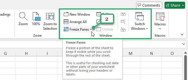
Step 2) In the Window group, click the Freeze Panes button.
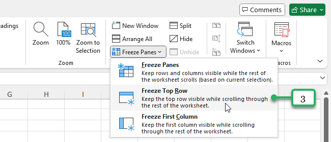
This will show you three options: ‘Freeze Panes’, ‘Freeze Top Row’, and ‘Freeze First Column’.
Step 3) Select the ‘Freeze Top Row’ in the options.
Easy as 1-2-3!
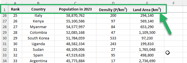
You’ll notice a darker grey line below your header row. It’s the indication that your top row is frozen. 👀

When you scroll even to the 30th or 40th row, you’ll still be able to see the top row of your worksheet.
How to Freeze Multiple Rows in Excel
In the case you want to freeze multiple rows in your worksheet, you can do that too.
Let’s say, you want to freeze the 2 top rows. ❄
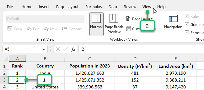
Step 1) Select the row (or the first cell in the row) right below the last row you want to freeze.
Since we want to freeze rows 1 and 2, click cell A3 in column A. There are 2 rows above this cell.
Step 2) Go to the View Tab.
Step 3) In the Window group, click Freeze Panes.
Step 4) Select Freeze panes in the options.
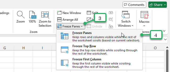
Now the dark grey line appears below Row 2 which means the top 2 rows are locked or frozen. When you scroll down through our Excel worksheet, the top 2 rows are visible. 👀

This is great when you’re comparing a certain criterion or data with the rest of the rows. ✅
Unfreeze Locked rows in Excel
To unfreeze the locked rows in your Excel worksheet,
Step 1) Go to View Tab.
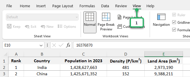
Step 2) Click the Freeze Panes button.
Step 3) Select Unfreeze Panes. This will unlock all rows and columns to scroll through the entire worksheet.
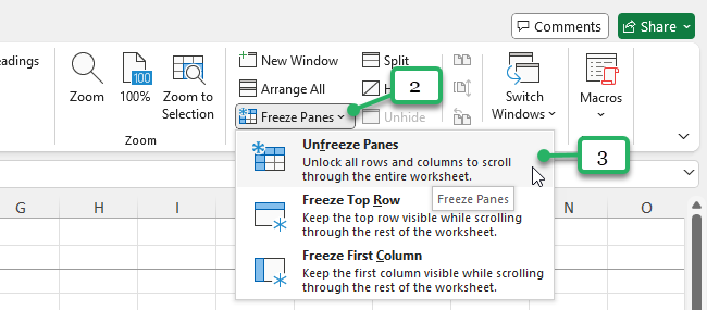
The dark grey line disappears and your first rows are unlocked.
That’s It—Now What?
Awesome! 🙌
With the Freeze Panes feature in Excel, you can keep the top row visible as you scroll through your Excel sheets.
Aside from freezing rows, you can freeze multiple columns too! Learn more about this in our Freeze Panes in Excel article.
Here are related Excel tutorials you can learn next: 💡
