How to Make a Weighted Average Formula in Excel
This article will take you back to the good times of fourth grade.
We all know what average is and how is it calculated. However, there is a better variation to the simple average function – the weighted average.
The weighted average goes a step ahead of the normal average. It not only averages the given numbers but also assigns them their corresponding weights.
To learn all about calculating weighted averages in Excel – continue reading the article below. 😀
Download our free sample workbook here to follow the examples used in the guide below.
Table of Contents
Weighted average formula
First thing first, what is the weighted average?
You will understand this by looking at the weighted average formula.
Here’s some data for when you go grocery shopping.
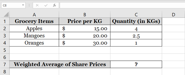
The grocery items list includes apples, mangoes, and oranges. All have different prices per kg.
So, for all these grocery items, what is the weighted average price per KG?
A different quantity of each item is bought. So, to find the weighted average we must multiply each item by its weight.
This means, multiplying each grocery item by its quantity.
1. Write the formula as follows:
= SUM (B2*C2, B3*C3, B4*C4)
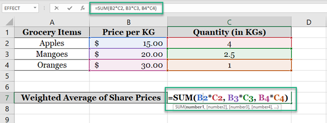
The results are as follows.
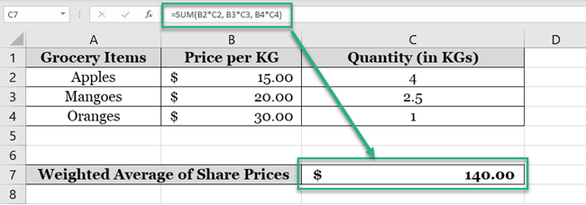
Here, we have multiplied the price of each grocery item by its quantity. And then we summed up all these values.
2. Divide the above formula by the total quantity of grocery items (which is the sum of their quantities).
= SUM (B2*C2, B3*C3, B4*C4) / SUM (C2:C4)

Here are the results.
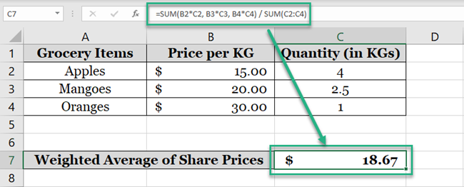
The $18.7 shows the weighted average price of all the grocery items.
Here’s a quick revision of the generic formula for weighted average.
= Sum of all values multiplied by their weights / Sum of all the weights
Weighted average vs. normal average
How is the weighted average different from the normal average? Why was it even needed?
Here’s the answer to this. 😄
The image below has the data for shares of three companies.
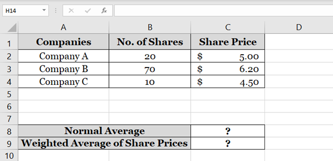
The data above shows the portfolio of an investor. It contains the number of shares and share price both.
What is the average share price of his portfolio?
Simply, put together the average function as shown below.
- Write the AVERAGE function as.
=AVERAGE (C2:C3)
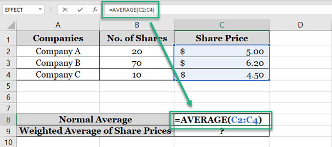
2. This results in a simple average of these three share prices.
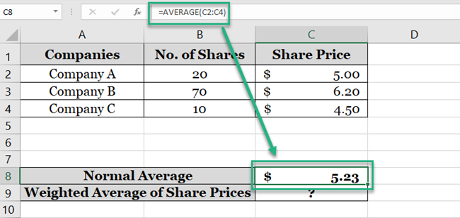
But? Does this number rightly represent the average share price for this portfolio?
No. Because we have a different number of shares of each Company. Hence the weight of each share price is different.
3. To calculate the weighted average share price, create a new column.
4. Write the following formula to multiply the number of shares of each by the share price.
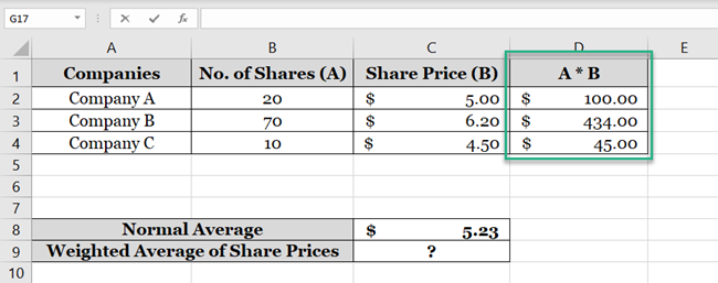
5. Calculate the sum of the number of shares and the above column.
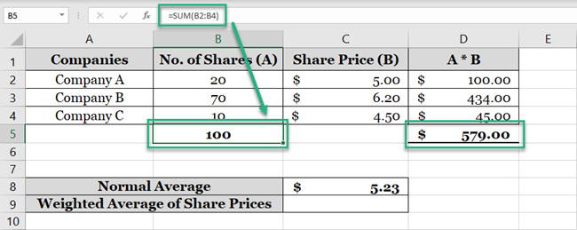
6. Calculate the average as follows.
= D5 / B5
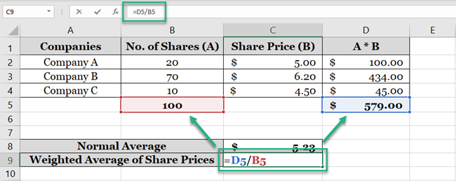
Where D5 consists of the sum of share prices multiplied by the number of shares. And B5 contains the total number of shares.
7. The weighted average comes as follows.
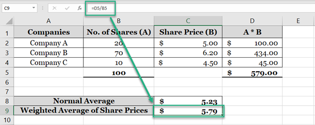
The answer takes a big shift. From $5.23 to $5.79.
This is how the weighted average varies from the normal average. It doesn’t only divide the sum of values by the number of values.
It weights all share prices (by multiplying them with the respective number of shares). And then divides the weighted share prices by the total weight (the number of shares).
With such data sets, the weighted average is considered much more precise than the normal average.
Weighted average with SUMPRODUCT function
Excel doesn’t offer a built-in function for calculating weighted averages.
However, the closest function for calculating the weighted average in Excel is the SUMPRODUCT function.
Let’s take the same example as above. To find the weighted average of share prices above follow these steps.
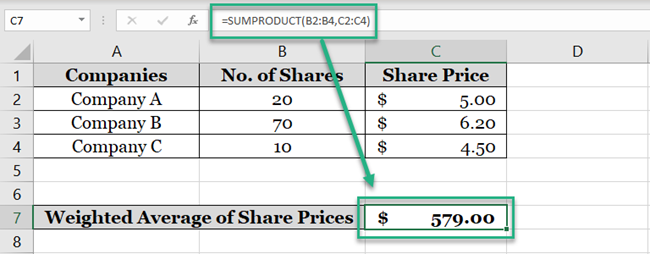
Write the SUMPRODUCT function below.
= SUMPRODUCT (B2:B4, C2:C4)
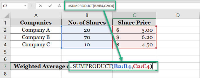
What does this function do? It adds up the cells in the range B2:B4 and C2:C4.
Next, it multiplies both these sums. That’s why we call it the SUMPRODUCT function. It not only sums two ranges but also multiplies their results.n).
To see the actual values being added and multiplied behind the above formula, press F9. The array values appear in the formula bar.
2. Here is the result of the SUMPRODUCT function.
3. Next, we need to divide it by the total number of shares.
4. To the above SUMPRODUCT function, add the SUM function as below.
= SUMPRODUCT (B2:B4, C2:C4) / SUM (B2:B4)
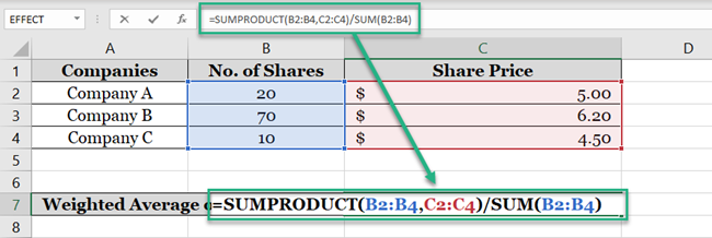
This divides the sum of the result of the SUMPRODUCT function by the SUM of the shares.
5. The weighted average comes out as follows. 😉
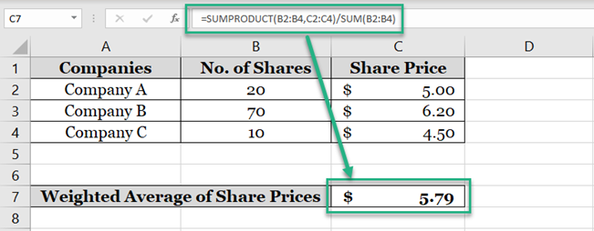
Must note that the results are the same from both methods. The SUMPRODUCT function and the manual calculation.
That’s it – Now what?
Although Excel doesn’t offer an inbuilt function for calculating the weighted average. But, there are still many ways how you may do it in Excel.
In the article above, we saw how you may set up a formula to calculate weighted averages in Excel. We also saw how the weighted average is different from the normal average. And how the results vary for both.
Lastly, there’s one way how you can combine two functions of Excel to calculate the weighted average. The SUMPRODUCT and the SUM function.
Helpful enough, the above functions are only a small part of Microsoft Excel. Some major functions that Excel is famous for, include the VLOOKUP, SUMIF, and IF functions.
Sign up here for my 30-minute email course to learn these functions (and many more) quickly!
Other resources
Did you find the above article interesting and helpful? If yes, we have plenty more for you.
Learn how to calculate simple averages in Excel. And also how to use some more advanced average functions like AVERAGEIF and AVERAGEIFS functions.
