How to Use the AVERAGEIF Function in Excel
The average is one of the most important central tendency measures of statistical distribution.
That’s fancy talk for: it’s an important metric that tells something about your data.
You calculate the average with the AVERAGE function 🧮
But with the AVERAGEIF function, you can add criteria to the average.
That means you can find the average height for a certain group of people (not just all the people), find the average sales for a specific product group, and much more. The possibilities are endless 💡
Let’s tune in on how to use the AVERAGEIF function, step-by-step.
Download the sample workbook here to tag along.
Table of Contents
How to use AVERAGEIF
The AVERAGEIF function has three arguments and the following is the syntax.
AVERAGEIF ( Range, Criteria, Average_range )
You can apply the function to the below example.
This example shows the region-wise sales details for a company that sells pens ✏️🖋️🖊️

Now let’s calculate the average sales for the “Pencils” product.
- Enter an equal sign and select the AVERAGEIF function.
=AVERAGEIF(

- Select the range where you need to check the criteria argument.
In this case, you have to check the criteria in the product column.
So, select the cell range in the product column.
Now your formula is;
=AVERAGEIF(B2:B10

- Enter the criteria.
The criteria for this case is “Pencils”.
You can enter numeric values, text values, and cell references as the criteria argument.
If you are entering a text value, enter it within quotes.
If you give a cell reference to an empty cell, the function treats it as a zero value 0️⃣
Now, your updated formula is;
=AVERAGEIF(B2:B10,”Pencils”

- Next, you have to enter the range in which you want to get numbers for the average calculation.
You have to give the cell reference to all the values in column C.
Then, the function should be;
=AVERAGEIF(B2:B10,”Pencils”,C2:C10

If any cell is blank or text value in the average range argument, the Excel AVERAGEIF function ignores it.
- Close the parentheses and press the “Enter” key.
Your complete formula is;
=AVERAGEIF(B2:B10,”Pencils”,C2:C10)
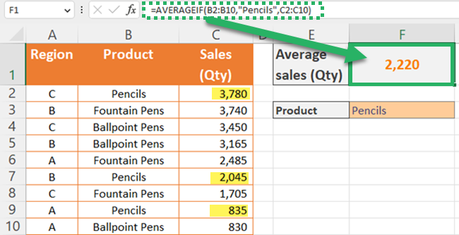
You get the average sales of pencils ✏️
Pro Tip:
Did you get a #Div! error value for the AVERAGEIF function? 😓
It can be due to one of these reasons:
- All the cells in the average range are blank cells or text values.
- No cells in the range of cells meet the criteria.
You can practice below each example to get more confidence.
AVERAGEIF formula examples
Here are some common AVERAGEIF examples to help you understand it better.
AVERAGEIF greater than (or equal to) or less than (or equal to)
Look at the below example. You have a new sales data set.

In the above example, you need to find average sales if sales values are greater than zero.
- Enter an equal sign and select the AVERAGEIF function.
=AVERAGEIF(

- Select the range.
You have to select all the values in the sales column.
=AVERAGEIF(C2:C10

- Enter the criteria for the function.
In this case, you have to enter logical criteria. You have to use logical operators for that.
Since you want to get sales greater than zero, you can use the logical operator “>”.
Use double quotes to enter criteria with logical operators.
The following formula is the updated function.
=AVERAGEIF(C2:C10,”>0″

Pro Tip:
The average range is an optional argument.
If you want to get the values to average from the range argument (first argument), you can omit the last argument.
- Close the parentheses and press the “Enter” key.
Now your formula is;
=AVERAGEIF(C2:C10,”>0″)
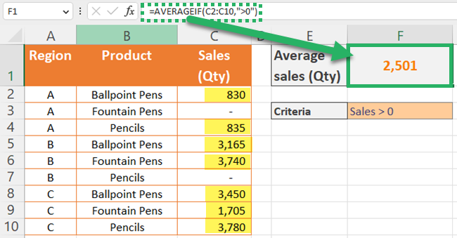
Pro Tip:
Assume you want to apply the criteria to separate cell range other than the range of cells in the first argument.
And you need to average cells not equal to zero.
Then keep the zero sales as empty cells.
The AVERAGEIF function ignores empty strings.
See the below example.
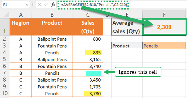
AVERAGEIF other column contains certain text values
With this function, you can average cells based on the partial match.
For that, you have to use the wildcard characters.
Use a question mark (?) to match any single character.
Use an asterisk mark (*) to match any sequence of characters.
When you need to find an actual question mark use a tilde (~) before it.
In the below example, you need to average all the values of pens.

- Enter an equal sign and select the AVERAGEIF function
=AVERAGEIF(

- Enter the range argument.
So, your formula should be;
=AVERAGEIF(B2:B10

- Enter the criteria.
You need to average of cells that meet the word “pens”.
Therefore, you can use an asterisk (*) sign before the word “pens”.
The updated formula should be;
=AVERAGEIF(B2:B10,”*pens”

- Enter the actual cells that you need to average.
So, select the range of cells in the sales column as cells to average.
Now, your formula is;
=AVERAGEIF(B2:B10,”*pens”,C2:C10

- Close the parentheses and press the “Enter” key.
You can see the following formula in the formula bar.
=AVERAGEIF(B2:B10,”*pens”,C2:C10)
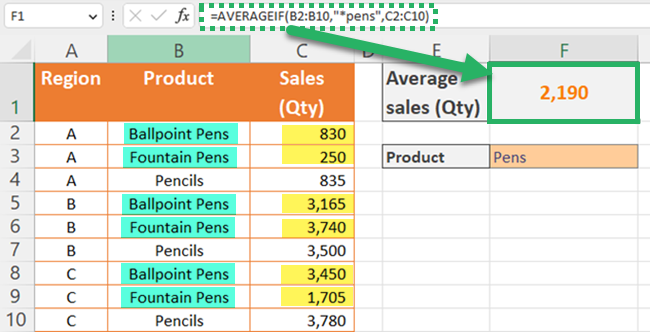
Now, you got the sales average of all pens 🖊️🖋️
AVERAGEIF Not equal to
Do you want to ignore certain cells in the criteria range for AVERAGEIF?
You can do that too!
Then you have to use not Not equal to (<>) in the criteria.
Look at the below example.

You can enter the same function as you entered in example 1.
However, this time you want to exclude the text with the given criteria.
So, you must enter the “Not equal to” sign before the criteria.
Your formula should be;
=AVERAGEIF(B2:B10,”<>Pencils”,C2:C10)
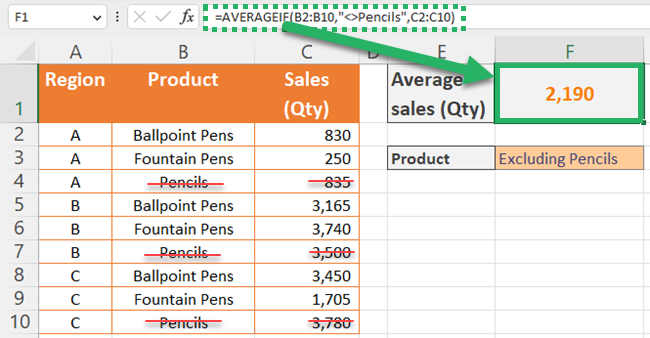
You get the sales average other than pencils 🚫✏️
Pro Tip:
When you enter the third argument of the AVERAGEIF function, you can enter only the upper left cell of the average range.
Excel will automatically consider the same size range of cells as per the given range of the 1st argument.
For example, if you enter =AVERAGEIF(B2:B10,”*pens”,C2:C4), AVERAGEIF returns the result for =AVERAGEIF(B2:B10,”*pens”,C2:C10).
That’s it – Now what?
Well done! 🥳
Now you know how to use AVERAGEIF with logical operators and wildcard characters.
As a result, you may use the AVERAGEIF function in a more dynamic manner, avoiding extra steps in your Excel calculations.
The AVERAGEIF function in Microsoft Excel is only one of many helpful functions.
VLOOKUP, SUMIF, and IF functions are among the other most commonly used and helpful functions in Excel.
Do you want to start learning these functions right away? 🧑🏻🎓
Enroll in my 30-minute free online course where I walk you through these Excel advanced features.
Other resources
When you need to apply more than one criterion for the average calculation, use the AVERAGEIFS function 🤹🏻
You can also use the SUMPRODUCT function to get the conditional average.
If you need to get the conditional total or count, read our articles about SUMIF and SUMIFS and COUNTIF and COUNTIFS.
If you want to learn more about wildcard characters, read our article about How to Use Wildcards in Excel ❔*️⃣
