How to Insert a Slicer in Excel Pivot Table
We occasionally filter data when building Pivot tables.
However, the user may not easily understand what is specifically filtered if the data is filtered using the report filter option 😵
The best Excel solution for this issue is to insert slicers. Slicers are visual filters of Excel. They make it easy for you to change your pivot tables with just a single click.
In this lesson, learn all about Excel slicers and how they can powerfully filter your pivot data table and charts 😀
Let’s go! Download the attached sample file to practice with me.
Table of Contents
Add slicer in pivot table
Adding slicers in Excel is very easy.
You can insert slicers into Excel Tables, Pivot Tables, and Pivot Charts 📈
The below Pivot table shows sales data.
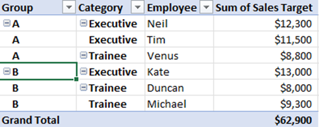
Imagine that now you want to insert a slicer into your Pivot table.
- Select any cell in the Pivot table and go to the Insert Tab.
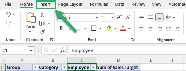
- Click slicer in the Filter group.

- Select a Pivot Table field that you want to add for the slicer from the insert slicers dialog box.
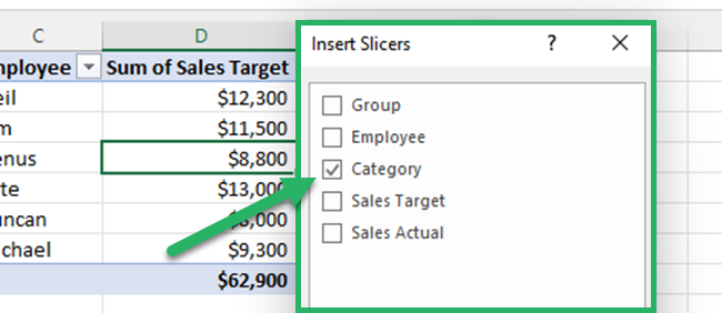
- Click OK to insert the slicer into the Excel Book.

Now you have added a slicer to your Pivot Table.
To filter data, you have to click the slicer button on the slicer.
If you select “Executive” from this slicer, the Pivot table data will be filtered to “Executive”.

Pro Tip:
Do you like to create a dynamic pivot chart?
Insert slicers for the chart. When you click the buttons of slicers, the Pivot chart will change automatically.
If you want to select multiple items, first, click on the multi-select button.

Click the clear filter icon to clear the slicer filter. You can see that icon in the upper right corner of each slicer.

You can customize these Excel slicers.
First, select the slicer to activate the Slicer tab.
If you are using Excel 2010, 2013, 2016, and 2019, you will see the Slicer tools tab with the slicer tools option tab instead of the Slicer tab.
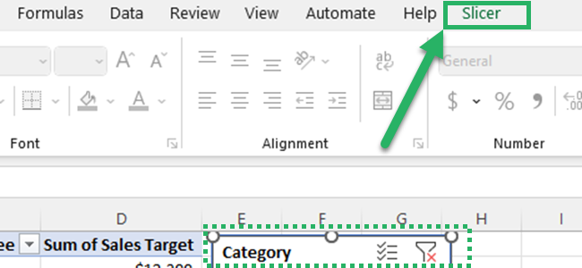
You can change the display settings of the slicer by clicking the slicer settings in the slicer group.

The slicer settings dialog box can be used to do the following customizations to the Excel slicer.
- Uncheck the box of the display header option to hide the slicer header.

- Change the caption of the slicer header.

- Sort the items on the slicer.

- Filter the items on the slicer.

You can use the slicer styles group to change the slicer style. You can select any of the Excel in-built slicer styles or you can create your own slicer style.

You can increase the number of columns and add multiple columns to the slicer.

If you want, you can adjust the size of the slicer buttons from the buttons group.

Add multiple slicers to the same pivot table
You can connect multiple slicers to the same Pivot Table as well.
All you have to do is to select more than one item from the insert slicers dialog box 🤹🏻
You can select “Group” and “Category” from the insert slicers dialog box in this case.
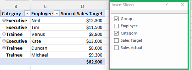
Then you will get multiple slicers to filter data in your Pivot Table.

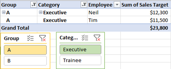
If you have selected “A” from the “Group” slicer and “Executive” from the “Category” slicer, your Pivot table will be filtered like below.
Use the same slicer for multiple pivot tables
You can even use a single slicer for multiple pivot tables or multiple pivot charts.
Assume that you have created 2 separate Pivot tables for sales data. One is for sales target and the other one is for sales actual.

You can connect these 2 Excel Pivot tables with one slicer.
- Create a slicer for the first Pivot table.
So, you can add a slicer for the group field of the sales target Pivot Table.
You can follow the same steps to create a single slicer.
Then, you can see your Pivot tables and slicer as follows.

- Go to the slicer tab after activating that by selecting the slicer of the first Pivot table.
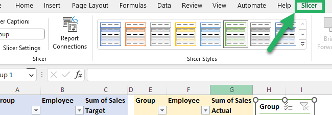
- Click report connections in the slicer group.

- Select the second pivot table that you have created from the Report connections dialog box.
Then, click OK.
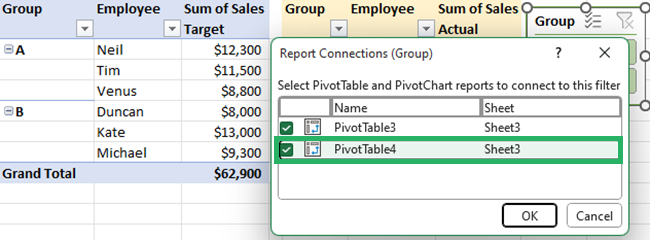
Now you can use this one slicer for both target sales and actual sales Pivot tables.
If you select “A” from this slicer, all the Pivot tables will show only Group A details.

That’s it – Now what?
Awesome! You now know all about Slicers in Excel. They are such a super cool feature for you to filter data in your Pivot Table and Pivot charts. Excel helped you do all that with just a few clicks 😀
If accomplishing a lot of tasks with just a few clicks is what you want, then Excel VBA is definitely the answer. With Excel VBA, you can unlock 🔓 Excel’s potential to work for your automation and a whole lot more. You can even automate your slicers with VBA.
Start learning VBA simple, easy, and free when you join my FREE Excel Expert VBA training.
Other resources
Did you know that adding slicers in Excel will make your dashboards more dynamic? Yes, you read that right. Apply what you’ve learned today and make your dashboards come alive 👍
Learn how to make dashboards in Excel, here’s our step-by-step guide (check out the 6 best dashboard templates I’ve found too).
You can also read more about Excel Tables and Pivot tables to organize, manage, and visualize your data without breaking a sweat 😏
