How to Insert a Checkbox in Excel
(4 Uncomplicated Steps)
If you want to collect user input in your spreadsheet there’s no better way than the checkbox.
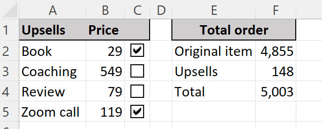
User-friendly, slick-looking, and easy for you to work with. Well… After you learn it at least.
If you’re having a hard time understanding the ins and outs of checkboxes, look no further.
Whether you’re into looks or functionality, this tutorial guides you through everything step-by-step.
If you want to tag along, please download my sample data workbook here.
Let’s dive in🤿
Table of Contents
Adding the Developer tab to Excel
There’s only one way to create a checkbox in Excel, and that’s from the Developer tab.
So, if you don’t see the Developer tab in your Ribbon already, you need to insert it first.
1. Click File on the Ribbon, and then click Options.
2. Click on ‘Customize Ribbon’.
3. Make sure there’s a checkmark in the Developer checkbox (kinda meta, right?)
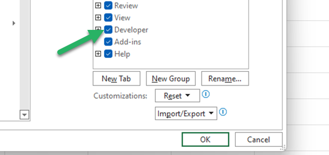
Click OK and now the Developer tab is visible from the Excel Ribbon.
How to insert a checkbox (in 4 steps)
In the worksheet, we have a small list of upsells.
In this list, a salesperson or the customer should be able to easily select the relevant upsells to the order.
And Excel checkboxes are the perfect tools for that.
Eventually, we want that list to be able to calculate the total upsell price automatically, based on the selections. But, let’s save that for later and start with just getting the checkboxes into the spreadsheet.
Step 1. Go to the Developer tab (here’s how to add it) and click on the down-arrow below the Insert button.
Step 2. In the drop-down that appears, pick the Check Box form control.
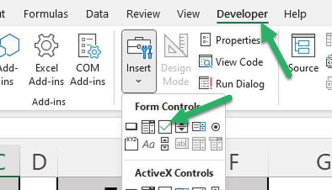
Don’t select the ActiveX Check Box control. The reason why is complicated but for 99% of checkbox creators, the ‘Form Controls’ Checkbox is more than enough👍
Step 3. Insert the checkbox by dragging its outline in your spreadsheet somewhere.

Step 4. Change the name and size of the checkbox, and move it so it fits what you’re trying to achieve.
The checkbox doesn’t have to have a visible name. You can just double-click the name and delete it, and make the checkbox all small like this if you want.
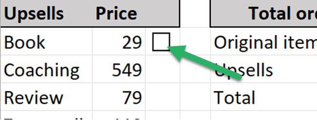
Voila! Now the user (and you) can left-click the checkbox to put a checkmark in it🙌
Insert multiple checkboxes in Excel
Now, you’ve learned how to insert a checkbox in Excel.
Easy peasy lemon squeezy🍋
But in many cases, you want to insert multiple checkboxes.
You do that by first inserting one checkbox, and then copying either the checkbox or the cell that contains the checkbox.
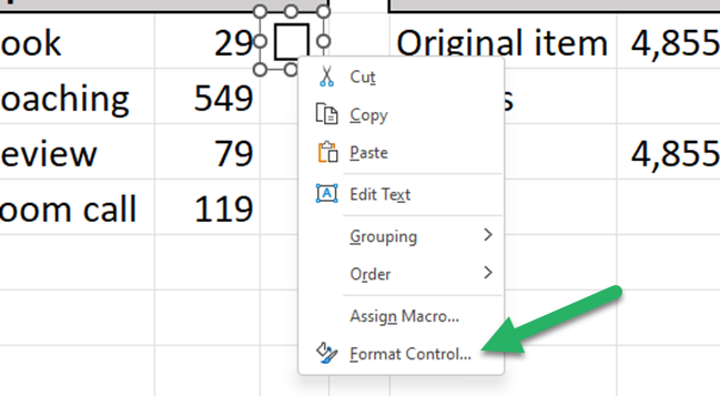
1. After you’ve inserted a checkbox, right-click it and select ‘Format control’.
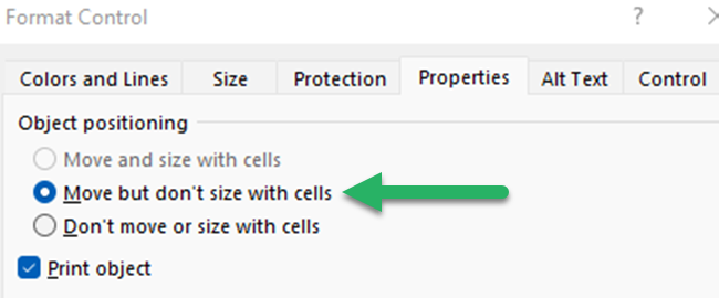
2. In the ‘Format Control’ dialog box go to the Properties tab.
3. Make sure the middle option ‘Move but don’t size with cells’ is selected and click OK.
4. Now, copy (or drag) the cell containing the original checkbox anywhere you want it.
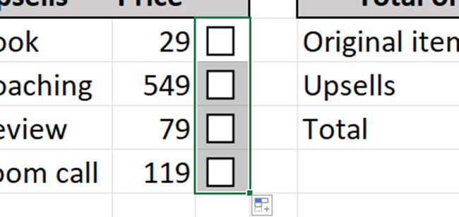
Visually, the upsell list is complete👏
Users are now able to indicate which upsells they want.
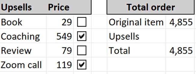
BUT this doesn’t do anything but visually indicate the user’s choices.
By linking the checkboxes to cells we can make it calculate the upsells total automatically.
How to link checkboxes to cells
Now, this is where the fun begins.
A visual checkmark in a checkbox doesn’t allow for any calculation. It’s pure visuals.
But you can link the checkbox to a cell so it displays a TRUE or FALSE value when it’s checked or unchecked.
It’s basically like making a cell reference.
1. Right-click on the first checkbox and click ‘Format Control’
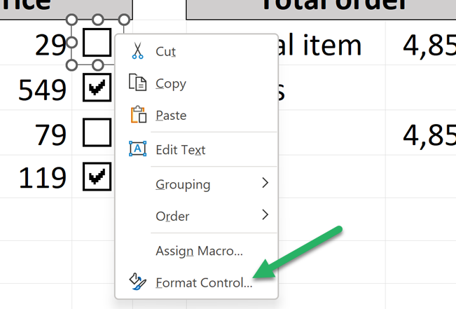
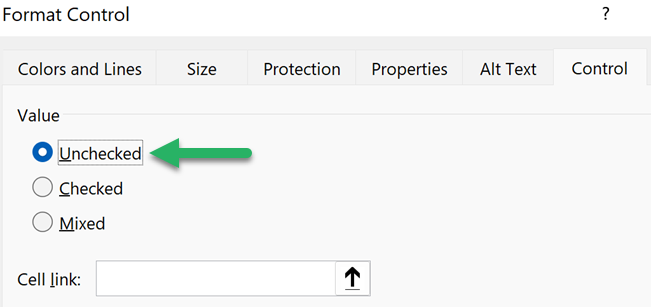
2. In the ‘Format Control’ dialog box, go to the ‘Control’ tab.
3. Select the ‘Unchecked’ option (radio button). That ensures the checkbox is unchecked by default when you open the spreadsheet containing it.
If you want the checkboxes to be checked by default, then select that option instead🕵️♂️
4. In the ‘Cell link’ box make a reference to the cell you wish to display either TRUE or FALSE depending if the checkbox is checked or unchecked.
Checked = TRUE, unchecked = FALSE.
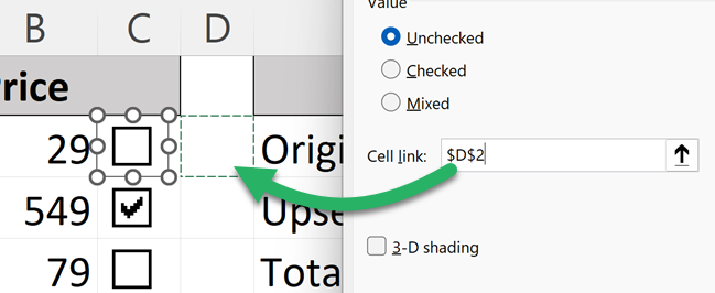
5. Do the same for all the checkboxes.
It should look like this by now.
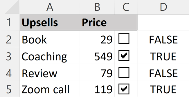
If the FALSE (or TRUE) values don’t show, try checking and unchecking the checkboxes a few times.
Now, all you need is a formula that adds up the upsells.
6. Write the formula:
=SUMIF(D2:D5, “TRUE”, B2:B5)
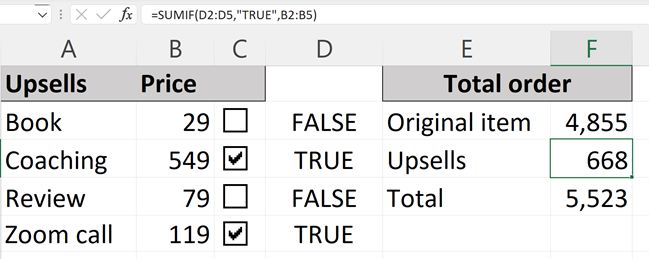
And that’s it!
Your interactive user interface now adds up the upsell prices from the chosen upsells. All are selected by checking and unchecking cool-looking checkboxes.
Well done💪
To make this look prettier, change the font color to white on all the linked cells.
Conditional formatting based on checkboxes
Now that you have established a cell link from the checkbox to the cell, you can do lots of things with it.
You can even use conditional formatting to add some visual interactivity.
That could be something like highlighting the text if the checkbox is checked. This works quite well when you have multiple checkboxes.
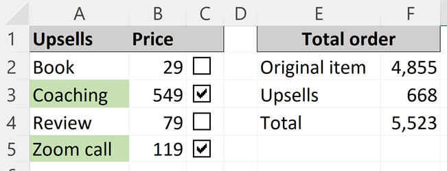
Let’s try that.
1. If you haven’t already, insert cell links from your checkboxes.
2. Select the titles of the items, in A2:A5, and click ‘Conditional formatting’ on the Home tab.
3. Click on ‘New rule’ and select ‘Use a formula to select which cells to format’.
4. Type the formula: =D2=TRUE
5. Define the format you want to apply if the formula is true and press OK.
Now, the upsell names are highlighted when the checkbox is checked – all due to linked cells.
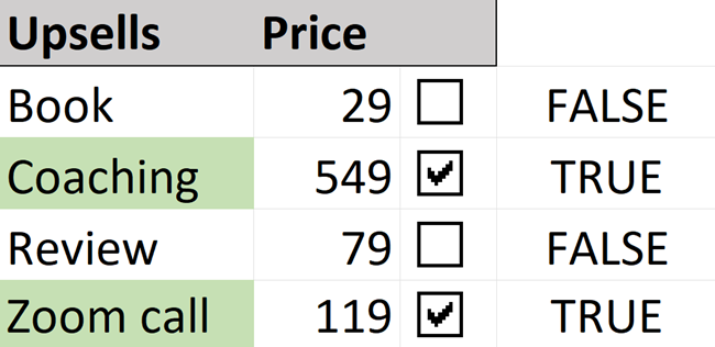
How to format your checkbox
If you want to make your checkbox look a little cooler, you can format it (almost) any way you want to.
Note that this formatting is static (normal formatting) and not dynamic (conditional formatting).
1. Right-click your checkbox and click ‘Format Control’.
2. In the control dialog box, go to the ‘Colors and Lines’ tab.
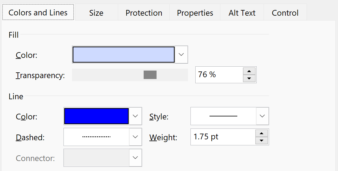
3. Choose the formatting you want and press OK.
And if you’re feeling crazy, you might end up with something like this🎉

How to insert a checkbox without the developer tab
- Select the cell where you want to insert the checkmark.
- Go to the Insert tab in the ribbon.
- Click on Symbol.
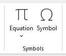
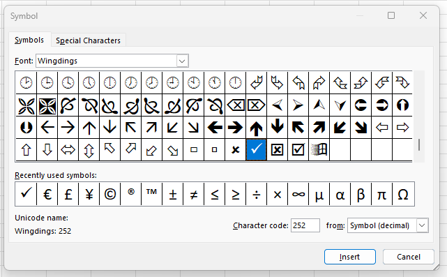
- In the Symbol dialog box, set the font to Wingdings.
- Scroll all the way to the bottom to find the checkmark symbol (you will find a checkmark in Wingdings at character code 252).
- Select the checkmark and click Insert.
- Click Close to exit the Symbol dialog box.
And there you have it, a checkmark without using the developer tab 🙂

Because it’s a font, you can style its color, background, size, etc., just like you would with other fonts.
Video: How to insert checkboxes in Microsoft Excel
Watch this video to learn how to insert a checkbox in Excel in just a few minutes.
You may also like
As I showed you in this guide, conditional functions such as IF/IFS and SUMIF work very well with a checkbox in Excel.
If you want to geek out on the possibilities in the developer tab, read more about it here.
Also, if you don’t need an actual checkbox but just the checkmark symbol, you can read up on that here.
Frequently Asked Questions
If I didn’t answer all your questions in the guide, please have a look below. Maybe you’re lucky🤞
