How to Add Error Bars in Excel: Step-by-Step With Examples
It is really challenging to ensure 100% accuracy for all of our data points when we present data.
In Excel charts, you can add error bars to reflect the degree of uncertainty in each data point.
Luckily, adding and modifying error bars in Excel is a piece of cake 🍰
Let me show you how it’s done, step-by-step!
You can download the attached Excel workbook to practice.
Table of Contents
How to add error bars in excel
I have created a bar chart for my data set.
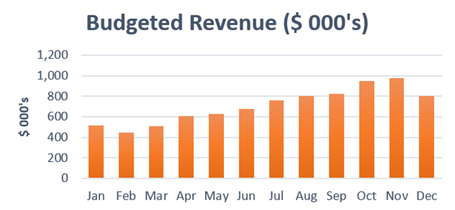
You can create any of the below Excel charts to add error bars.
- Bar chart
- Line chart
- Bubble chart
- Column chart
- Scatter chart
- 2D area chart
If you wish to add horizontal error bars, you have to create bubble charts or scatter charts.
Let’s add error bars to our chart.
- Click on the chart to select the chart.
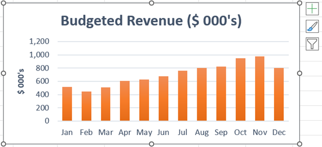
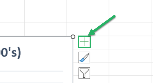
- Click the chart elements (+) button of the chart to expand the chart elements.
- Check the error bars box of the chart elements
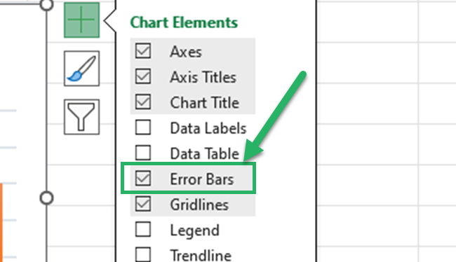
Error bars are quickly added to our Excel chart 🥳
These default error bars are standard errors of our data points.
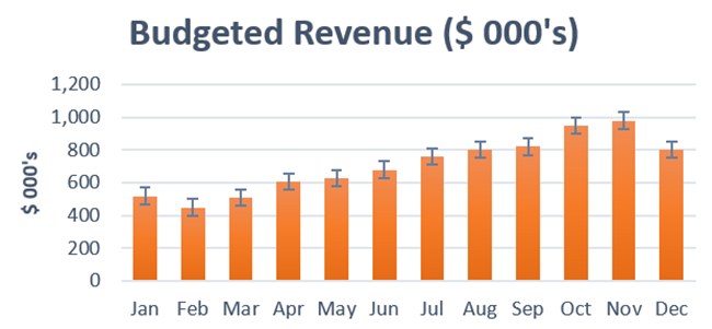
If you are using Excel 2007 or 2010, you have to follow the following steps to add error bars.
Select the chart to activate chart tools > Go to the layout tab > Select error bars from the analysis group.
If you need to show something other than a standard error, click the arrow next to the error bars.
You can select one of the predefined error bar options.
- Standard Error
- Percentage
- Standard Deviation
Or you can select More Options to create custom error bars.
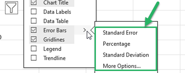
Excel will calculate the Standard Error and the Standard Deviation automatically for our data 😍
If you select the percentage error bar option, Excel will use 5% as the default value.
You can format error bars in your chart 🙂
- Click More Options from the error bars dropdown menu to open the format error bars pane.
Pro Tip:
Do you want to open the format error bars pane quickly?
Just double-click the error bars in Excel🖱️
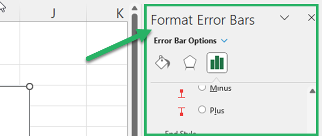
You can customize your vertical error bars or horizontal error bars as follows.
- Add your own error bar amounts for a fixed value, Percentage, or standard deviation.
First, click the radio button for the relevant error bar amount option. Then specify your own values in the box.
In this case, I am selecting standard deviation error bars and setting the standard deviation values to 0.75.
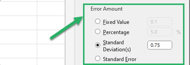
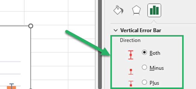
- Change the direction of the error bars.
You can select one of the below options.
Both – To show both positive error values and negative error values ➕➖
Minus – To show only the negative error values ➖
Plus – To show only the positive error values ➕
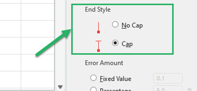
- Change the end style of error bars.
You can select either No cap or cap to error bars in your Excel chart.
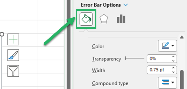
- Change the formatting of the error bars.
Select the fill and line tab to change the color, width, cap type, etc. of error bars in Excel.
What do error bars mean exactly?
Visual representations of data variability in Excel are called error bars.
They display the accuracy of a measurement.
It helps to learn how far the actual value could be from the known value or the given data point.
The error bars usually show the standard deviation and standard error.
Error bars in charts provide readers with a more thorough understanding of the data set.
Add custom error bars
Do you want to add custom error bar values? or custom values to each error bar in your chart?
You can do that too! 🎉
- Select the custom from the error amount options of the format error bars pane.
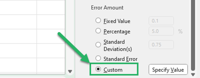
- Click the specify value button.
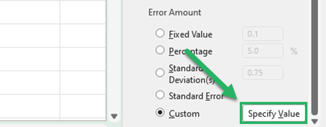
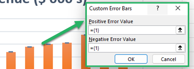
- Specify a positive error value and a negative error value for error bars in the dialog box.
You can enter different error values for individual error bars also. You can just type values for the individual error bars and separate them with commas.
If you want to remove error bars, enter zero in the relevant boxes. Don’t just keep it blank.
Pro Tip:
How can you add individual error bars dynamically?
Let’s say we have the budgeted negative revenue variation for each month.
Now we want to add these budgeted negative revenue variations as error bars of our chart.
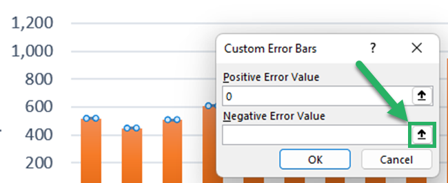
- Click the collapse dialog icon of the negative error value of the custom error bars dialog box.
Remember to change the positive error value to zero.
- Select the cell references and click “OK”.
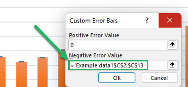
Now your custom values are displaying as error bars.
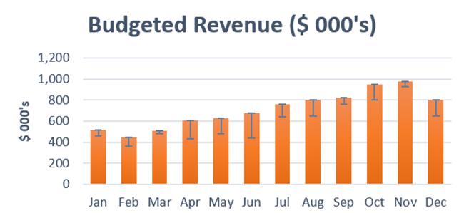
Whenever you change the given values, Excel will automatically update the error bars 👏🏻
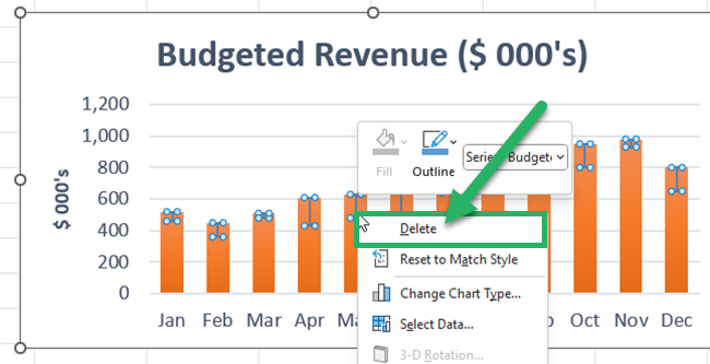
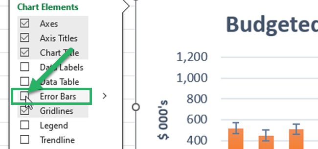
If you want to delete error bars in Excel, you can do it using one of the following methods.
- Select error bars. Then right-click and click delete.
- Uncheck the error bars from chart elements.
- Click the error bars and press the “Delete” button.
That’s it – Now what?
Well done! ✌🏻
Now you know how to add, modify, and delete error bars in charts.
But charts (and especially error bars) are only a small part of Microsoft Excel 🤔
To make the most out of Excel, mastering functions like VLOOKUP, SUMIF, and IF is essential.
My free 30-minute online Excel course will help you learn them in no time. Register now! 🧑🏻🎓
Other resources
Read our articles about how to create Line Graphs, Column Charts, and Scatter Plots to refresh your knowledge about Excel graphs 📈📊
If you like to add a trendline also to your chart, read our article about How to Add a Trendline in Excel.
