How to Use AutoSum in Excel: Button and Shortcut
If Excel can help you with complex calculations and data analysis, then solving for the SUM in Excel is a piece of cake 🍰
The SUM function is so popular and widely used that Microsoft Excel decided to add a special button for it in the Excel Ribbon: the AUTOSUM button 😀
Now, you can automatically get the SUM in a few clicks.
In this article, you’ll learn all about the Excel AutoSum function and how to use it.
Learn it first-hand by downloading this workbook with sample data you can work on 👍
Table of Contents
How to use Autosum in Excel
The AutoSum in Excel is such a helpful button when you want to sum numbers in your Excel columns or rows quickly.
When you click AutoSum, Excel automatically enters a SUM formula to sum numbers.
See how the AutoSum formula works firsthand.
Open your practice workbook. You’ll find that you need to complete the data table by getting the sum or total per column and row.

Don’t worry! With the Excel AutoSum feature, you’ll complete this table in no time 😊
Say you want to sum the monthly sales first. To do that…
- Select the cell next to the numbers you want to sum.
Since we want to sum a column, select the cell immediately below the last value in the column. In our case, select cell B7.

- Go to the Home Tab.

- In the Editing group, click the AutoSum button.

A SUM formula automatically appears in the selected cell (B7), and a range of cells you want to add gets highlighted (B2:B6).
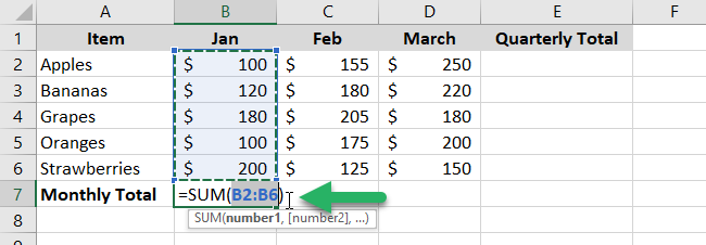
Just check if Excel selects the correct range to total 👀
In most cases, Excel selects the correct range to the total. But it’s always safe to check ✅
In a rare case when Excel selects a wrong range, you can correct it by manually typing the desired range in the SUM formula or by dragging your mouse cursor through the cells you want to sum.
If everything looks good to you,
- Press Enter to complete the formula.
Now, you can see the grand total in the cell. You can also see the SUM formula in the formula bar above.
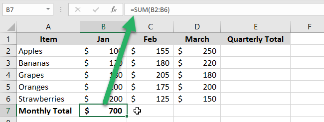
You can repeat the steps for the total monthly sales in the next columns. Or just drag the fill handle to the right 😉
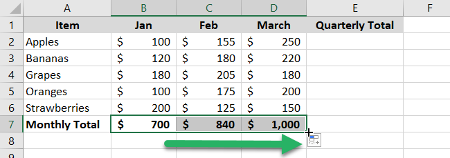
That was easy, right?
Well, there’s another way to do it.
Shortcut for inserting the SUM function
The fastest way to insert the SUM function is by using the AutoSum keyboard shortcut.
If you’re an Excel user who prefers working with the keyboard to the mouse, this method is for you. Plus, it’s always cool to know the shortcut 😎
It involves pressing two keys: the Alt key and the Equal sign (“Alt” + “=”).
Let’s do it.
This time, let’s get Apple’s quarterly total in our practice workbook 👇
- Select the cell where you want to insert the AutoSum formula.
In our practice workbook, it’s cell E2.

- Hold down the Alt key (Alt) then press the Equal sign (=) on your keyboard.

A SUM formula appears in the selected cell (E2), and a range of cells you want to add gets highlighted (B2:D2).

Just like what you did above check if Excel selects the correct range to total 👀
If it’s good to go,
- Press Enter to complete the formula.
Now, you can see the result in the cell and its SUM formula in the formula bar.

Drag down the fill handle to get the total for each item in each row. Nice work! 🎉

Pressing the AutoSum shortcut keys on your keyboard is exactly like pressing the AutoSum button on the ribbon. It does the same thing.
But there’s more to this AutoSum button than just getting the sum 🧐
AutoSum button with other functions
Apart from adding cells, you can use Excel’s AutoSum button to insert other functions.
What other Excel functions? 🤔 You’ll see.
- Go to the Formulas Tab.
- Click the Autosum drop-down arrow in the Function Library group.
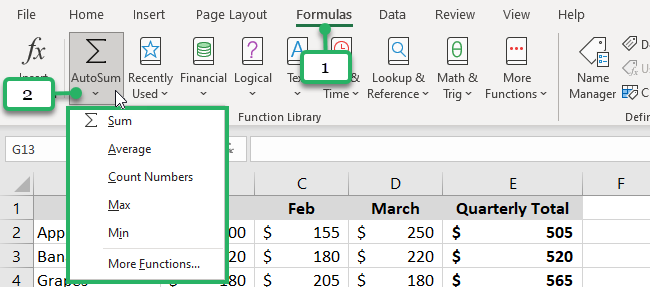
You can insert other functions such as:
- AVERAGE – to return the average (arithmetic mean) of numbers.
- COUNT – to count cells with numbers.
- MAX – to get the largest value in the selected range.
- MIN – to get the smallest value in the selected range.
All you need to do is select the cell where you want to insert any of these formulas and click the AutoSum drop-down arrow, and choose your desired function from the list.
Let’s break down two of these Excel functions: SUBTOTAL and AVERAGE.
AutoSum with subtotal function
You can use the AutoSum feature to create formulas with the SUBTOTAL function.
The SUBTOTAL function can perform a range of functions on a filtered part of a list or a database.
First, you need to apply a filter to the range. To do that…
- Right-click the column headers.
- Select Filter from the right-click menu.

- Select Filter by Selected Cell’s Value.

Now, your data table will look like this.

Don’t worry, you’re on the right track!
Say you only want to sum up the January monthly sales for three items: Apples 🍎, Bananas 🍌, and Grapes 🍇.
By saying that, you only want the SUBTOTAL.
- Select the filter button.

- Select Apples, Bananas, and Grapes.
- Click OK.
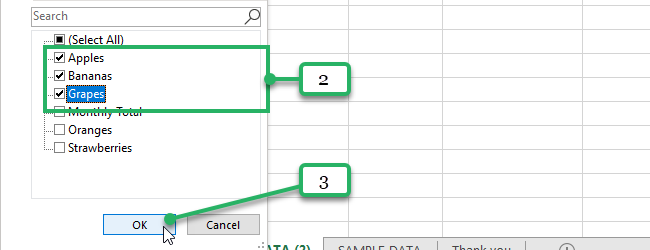
Your table only shows what you filtered.

Now, we can solve the SUBTOTAL. Follow these three easy steps: 👇
- Select a cell in the column or the first empty cell below the filtered range.
- Click the AutoSum button or press the AutoSum shortcut (“Alt” + “=”).
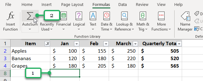
A SUBTOTAL formula will appear in the cell.
- Make sure you highlight the correct range.
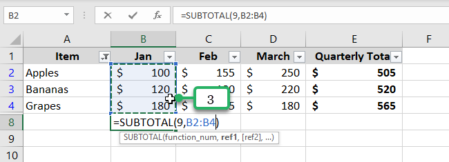
- Press Enter.
A SUBTOTAL is now calculated.

The advantage of using the SUBTOTAL formula is that it only displays the sum of the visible rows only.
Amazing, right? 😀
AutoSum with average
Sometimes, when we need to calculate the SUM, we also need to solve for its AVERAGE.
Just like calculating for the SUM, it’s easy to solve the AVERAGE too as it follows the same steps.
- Select a cell below the column or to the right of the row of numbers for which you want to find the average.

- Go to the Formulas Tab.
- Click the AutoSum drop-down button in the Function library group.
- Select Average.
An AVERAGE formula is inserted in the cell. Make sure it highlights the correct range.
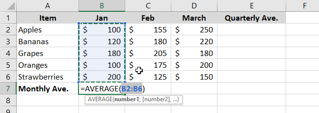
- Press Enter.
And there you have it! 🙌

That’s your January monthly sales average.
That’s Excel doing the math for you! 😉
PRO TIP:
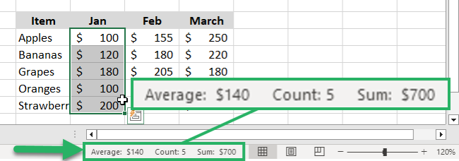
If you want to quickly know the SUM, AVERAGE, and COUNT of your data, Excel’s Status bar got you covered.
When you highlight cells with numeric data, the status bar in Excel shows you quick information like this.
Super cool, right?
That’s it – Now what?
Way to go! You can totally let Excel do the math for you 😊
With the Excel AutoSum button, you can solve for the SUM, AVERAGE, COUNT, and many more in a matter of a few clicks.
If these basic functions are too easy for you and you’re looking for a good challenge, then you can level up your Excel skills by learning advanced Excel functions 🚀
My three best recommendations? Start on VLOOKUP, IF, and SUMIF functions.
Allow me to save you some time and energy 😉
Join my Excel Intermediate Training 💻 to learn all of these in the most comprehensive way and all for FREE!
Other resources
Want an in-depth lesson about the basic functions mentioned above? 🤿
Read each article about the AVERAGE, SUBTOTAL, COUNT, and MIN & MAX functions we’ve written for you.
Don’t miss out on learning how to filter in Excel as well.
