How to Create Macros in Excel: Step-by-Step Tutorial (2024)

Get ready to have your mind blown! 🤯

Because in this tutorial, you learn how to create your own macros in Excel!

That’s right! And you don’t need to know VBA (Visual Basic for Applications)!

Instead, you will use the Excel macro recording feature to send your spreadsheet experience into overdrive! 🚀

So, read on and try it out yourself using this practice Excel workbook.

What are Excel macros?

A macro is a small program or set of actions that you can run repeatedly. Excel macros are used to automate repetitive tasks to save a lot of time and hassle.

For example, open and take a look at the practice Excel workbook.

Businesses would often have lists like this one. These are potential customers they might want to reach out to and market their products.

Notice how Columns C to H are just pieces of information extracted from Columns A & B.
(Learn how to extract strings from texts in this tutorial!)

To streamline the worksheet, you can hide Columns A & B. You can also hide the rest of the columns on the right starting from Column I.

Let’s do this using Excel macros!

How to record Excel macros

1. Click on the View tab in the Excel ribbon

2. Next, click on the Macros button on the right side of the View ribbon

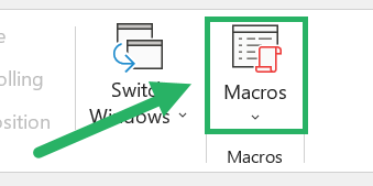
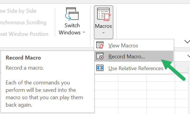
3. This will open the Macros drop-down.

Click Record Macro.

4. Enter a name for your macro, something like Hide_Columns.

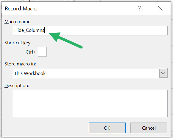
4. Select Store macro in: This Workbook then click the OK button.

Excel is now recording your actions to create a macro.

5. Select Columns A & B and then right-click on the highlighted Column Bar to Hide them.

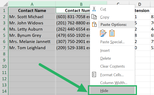
6. Then select Column I and press Ctrl + Shift + Right Arrow to include all remaining columns on the right.

7. Right-click on the highlighted Column Bar then click on Hide.

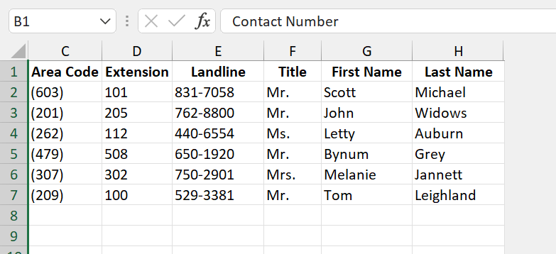
Your worksheet should now look like this:

To end the macro recording:

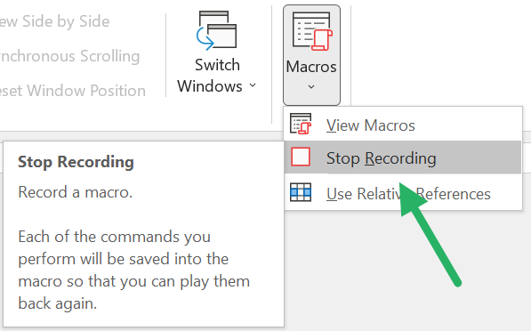
8. On the View ribbon, click on Macros and select Stop Recording.

Good job! 👏

You have created your first macro in Excel!

But wait, where is the recorded macro?

To view all of the available Excel macros :

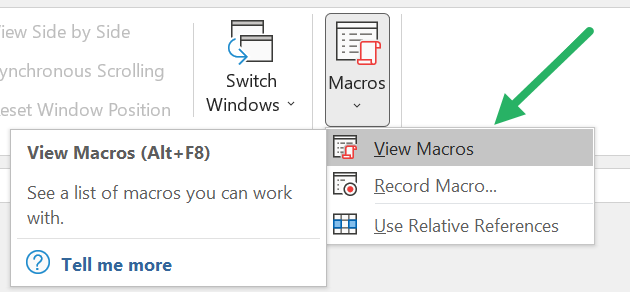
1. Select View Macros.

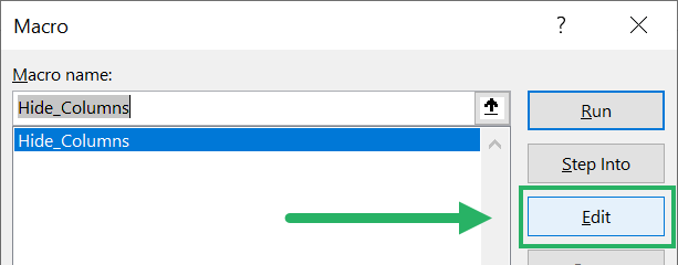
2. This opens the Macro window. Saved macros will be listed here and you can Run whichever one you need.

You can also click on Edit to view the VBA code window.

3. The VBA code editor opens.

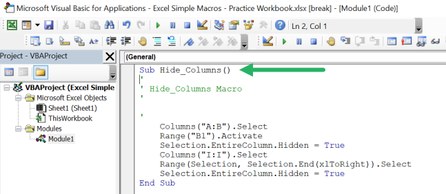
Notice the Hide_Columns Sub procedure. You don’t have to write or edit VBA code for the macro.

Excel automatically generated each code line based on the recorded keystrokes and mouse clicks.

The Record Macro feature is powerful enough for general spreadsheet automation needs.

But if you want to customize your own VBA macro, you can learn more about Visual Basic for Applications (VBA) here.

Using the Developer tab

Let’s record another macro to Unhide the hidden columns.

This time, you can record the macro from the Developer tab.

The Developer tab gives you access to a lot of useful Microsoft Excel features such as the Visual Basic Editor. It also allows you to quickly insert form controls such as buttons and checkboxes.

However, the Developer tab is not visible in the Excel ribbon by default.

To add it:

1. Right-click on the Excel ribbon.

Select Customize the Ribbon.

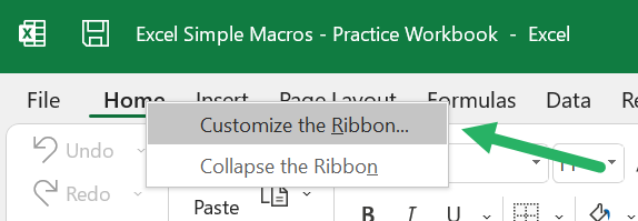
2. This opens the Customize Ribbon window.

On the right side, check the Developer tab checkbox.

3. You should now see the Developer tab.

To start recording the Unhide macro:

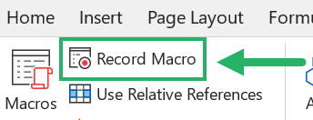
1. Click on the Record Macro button in the Developer tab.

2. Name this macro Unhide_Columns.

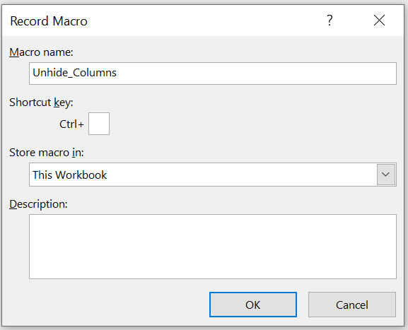
3. Click OK.

The recording has started.

4. Press Ctrl + A twice to select all cells.

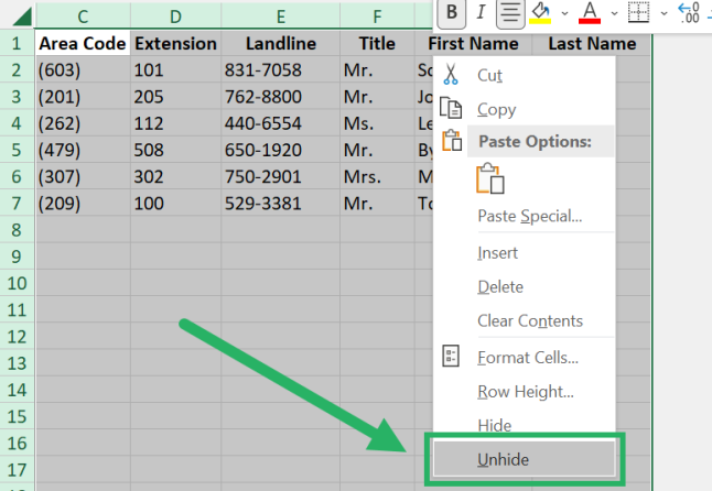
5. Right-click anywhere on the Column Bar then click Unhide.

6. Click on the Stop Recording macro button to finish up.

Great work! 👌

Now you have two recorded macros that can be executed.

How to run an Excel macro

To run your macros:

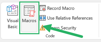
1. Click on the Macros button from the Developer tab.

2. In the Macro window, select the macro Hide_Columns and click on Run.

The macro executes the actions recorded earlier and hides the unnecessary columns.

You can also run macros from the View ribbon.

Run Excel macro from the View tab

This time, run the Unhide_Columns to show all the columns.

1. On the View ribbon, click the Macros button and select View Macros.

2. Select the Unhide_Columns macro and Run it.

This unhides all the columns in the worksheet.

As you can see, the Macro window allows you to quickly run all the available macros.

But you can execute them even faster by using buttons and shortcuts ❗

Run Excel macro from a button

For this next example, you will assign macros to buttons which will be located on top of the table.

1. Insert 2 rows above the table headers. Select Row 1 then press Ctrl + Shift + Plus Sign(+) twice.

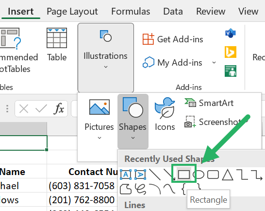
2. To create a button, click on Insert > Illustrations > Shapes.

Then select the Rectangle.

3. Draw a rectangle and format it as you’d like. Label it “HIDE”.

This will be your HIDE button. Place it between columns A & B so it will be hidden with the columns when the macro runs.

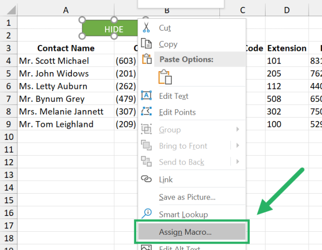
4. To assign a macro, right-click the shape and select Assign Macro.

5. In the Assign Macro window, select Hide_Columns and click OK.

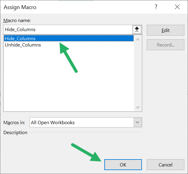
The Hide button now works!

Now, do the same for the Unhide_Columns macro.

6. Create another rectangle button and label it “UNHIDE”.

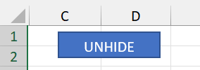
7. Repeat Steps 4 & 5 but this time, assign the Unhide_Columns macro.

Alright! 👍

Now you can quickly run your macros using the HIDE and UNHIDE buttons.

Run Excel macro from a shortcut key

It is sometimes better to run macros using a keyboard shortcut.

For this next example, you want to quickly highlight people on the list that expressed interest in the business.

To create a macro for this:

1. Select any cell within the table.

2. On the Developer tab, toggle ON the Use Relative References button.

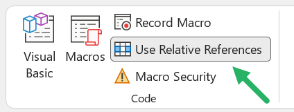
3. Start recording with the Record Macro button on the Developer tab.

Or, you can also click the Record Macro button on the Status Bar.

4. Name the macro Mark_Interested.

Then assign a shortcut key. For example, Ctrl + Q.

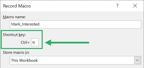
Click OK. The recording has now started.

4. Highlight the row of the Active Cell using the keyboard shortcut Shift + Space Bar.

5. Apply the formatting:

• Fill using the color Green
• Change font color to White

6. End the macro recording from the Status Bar

All done!

Try to use the shortcut Ctrl + Q to quickly apply formatting to entire rows.

Saving macro-enabled workbooks

If you save the practice workbook, this window will pop up:

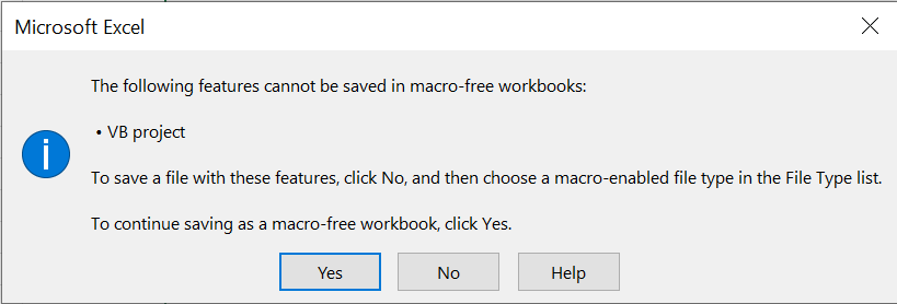
This is because the practice workbook is currently saved with the .xlsx file extension which does not support macro features.

To save properly, change it to the .xlsm file extension for macro-enable workbooks.

Keep this in mind when saving your work.

Congratulations! 🤩

You are now familiar with Excel macros.

Try to record your own macros and start saving time ⏱️ on your work!

That’s it – Now what?

The examples above are very useful though they are quite simple.

You can record macros for more complex functions. Such as creating custom charts or selectively copying rows of data to another workbook.

But recording and playing macros is just the tip of the iceberg.

With VBA programming, you get access to a whole different level of Excel automation. 🤖

And while Visual Basic may seem overwhelming at first, you can start slow with basic variables and IF statements. These are much easier than you might think!

Learn all that and much more in my free 30-minute online VBA course here.

Other resources

If you want to know more about the inner workings of the record macro feature, check out my Excel macro tutorial for beginners on YouTube.

You can also dive right into VBA by reading this article or watching this introductory video on VBA and macros!

Hope you enjoyed this article!