How to Square Root in Excel: Type Symbol and Calculate (2024)

Microsoft Excel is great for performing mathematical operations!

It’s one of the world’s most powerful calculators – at your fingertips.

One of these mathematical operations is finding the square root of a number.

Let me show you how it’s done in a few minutes ⏲️

If you want to tag along as you read, download the sample workbook here.

How to type square root symbol in Excel

In a written equation, the radical symbol (√) is used to denote the square root. But that symbol is not very common in Excel, right? So what should you use 🤔

That’s where the caret symbol (^) comes in 👏

In Microsoft Excel, the caret symbol (^) symbol stands for exponentiation. Exponentiation is a mathematical operation that raises the quantity to a power.

But unlike the radical symbol, using the caret symbol alone will not be enough to get the square root value. To find the square root using this method, we need to use the caret symbol with (1/2) or (0.5) as the exponent.

Why are we using 1/2 or 0.5 you ask?

That is because we are calculating the number to the power of a half. Which is equivalent to finding the square root 💡

1. Using the workbook provided, select cell B2 and type in =A2

2. Now, insert the caret symbol (^)

3. Complete the formula by adding 0.5 then press enter

As mentioned, you can also use 1/2 on the formula bar instead of 0.5. This is only a matter of personal preference but both methods will calculate the square root.

For example, type in the same formula but replace 0.5 with (1/2) in Cell B2

As shown in the above formula, we insert (1/2) instead of 0.5 and we got the same result. This only proves that whatever formulas we use, the square roots will be the same.

Pro Tip!

Note that Microsoft Excel will not get the square root of negative numbers. This is because the negative value does not have a square root. So if we try to calculate the square root of a negative, it will return the error “#NUM!” 😱

Calculate square root with SQRT function

Excel has created a specific function to perform this calculation. That is the Excel SQRT function.

It can calculate square roots without the need for extra numeric value! How cool is that 😎

SQRT function has only one argument which is the Number.

Number represents the base number on which the square root calculation is based from.

Now, let’s try using the SQRT function to calculate the square root.

Use column C on the sample workbook so that we can compare the result between the caret symbol and SQRT methods.

1. In cell C2, type in =SQRT(

2. Complete the formula by adding the cell reference A2. Add a close parenthesis ) right after the cell

3. Lastly, press enter

SQRT function is very straightforward and is a lot easier to use than the first method 💪

Same to the caret symbol method, SQRT will not accept numbers with a negative sign as shown in the below formula.

Calculate the square root in Excel with formula

Now that we understand both methods, it is time to incorporate those into a formula 👌

Let’s review the scenarios below and create the formula for each:

Scenario 1: Get the square root of a negative number

Real-life Mathematics and even Excel will not be able to get the square root of any negative number.

But there is a method that we can use to get the square root in Excel 😉

And that is converting the negative number to a positive number using the ABS function 😲

The ABS function returns the absolute value of a number without its sign.

This function has only one argument which is the Number. This is the source number that we will convert to positive.

Let’s do it first using the caret symbol method:

1. Select cell B4 and type in =ABS(

2. Put cell A4 as our reference and add a close parenthesis )

3. Insert the caret symbol ^

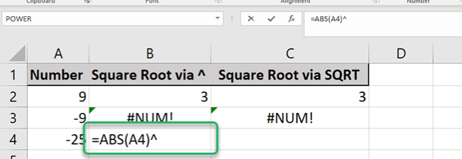
4. Complete it by adding 0.5 or (1/2). Press enter

Now, let’s try it using the SQRT function method:

1. In cell C4, type in =SQRT(

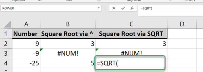
2. Add ABS( into the formula

3. Lastly, insert cell A4 with 2 close parentheses )) and press enter

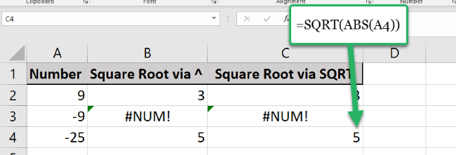
Excel can calculate the square root of the negative number using the above formulas 🤘

This became possible as the ABS function is converting the negative (-25) to positive (25).

And no matter what syntax was selected, Excel returns the square root correctly.

Scenario 2: Set a condition to calculate the square root if the data is a number

Let’s assume you are dealing with multiple data types and you need the square root of all the numbers in a table 😨

To do this, we need the help of two other Excel functions, ISNUMBER and IF.

ISNUMBER function checks whether data is a number, and returns TRUE or FALSE. It only has one argument which is the value, that represents the data we need to evaluate.

IF is an Excel logical function that checks whether a condition is met or not. It has three arguments:

1. Logical test – a logical expression that can be evaluated as TRUE or FALSE
2. Value if True – the value to return when logical_test evaluates to TRUE.
3. Value if False – the value to return when logical_test evaluates to FALSE.

We will be using the same table for this exercise

Let’s try using the caret method first:

1. Select cell B5 and type in =IF(

2. We will then add ISNUMBER(

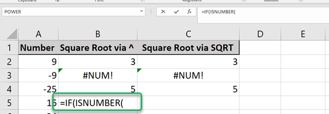
3. Put cell A5 as our reference and add a close parenthesis ) and a comma (,)

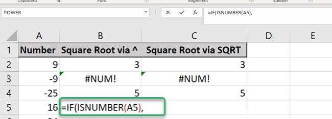
4. Insert the next argument by adding A2^0.5,

Looks familiar? This is the caret method we used before 😁

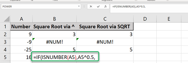
5. Complete the formula by adding a double quote (“”) which represents blank data.

Close the formula using a close parenthesis ) then press enter

It should look like this now: =IF(ISNUMBER(A5),A5^0.5,””)

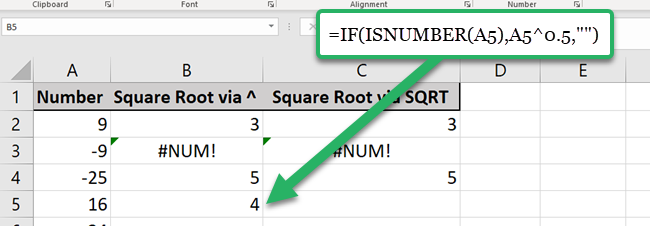
6. Copy and paste the formula until cell B8

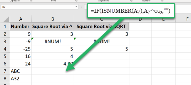
Let’s try it now using the SQRT function

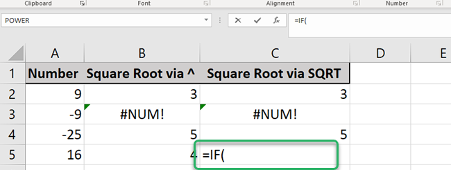
1. Select cell C5 under the dedicated column for SQRT and type in =IF(

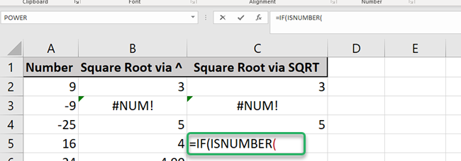
2. Next, insert ISNUMBER(

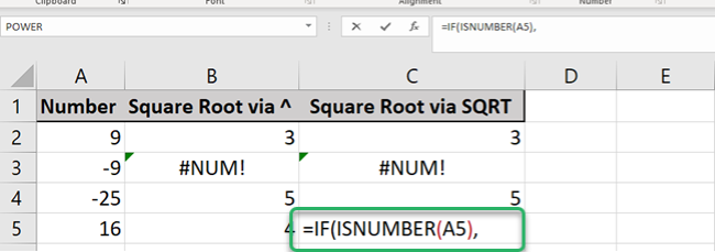
3. Add cell A5 as our reference and put a close parenthesis ) and a comma (,)

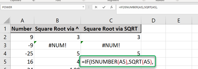
4. Complete the next argument by adding SQRT(A5),

Looks familiar again? This is the SQRT method we used before 😲

5. Complete the formula by adding a double quote (“”) which represents blank data.

Close the formula using a close parenthesis ) then press enter

It should look like this now: =IF(ISNUMBER(A5),A5^0.5,””)

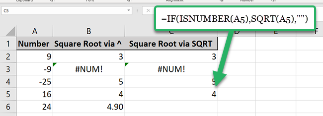
Whichever formulas you used, will provide the same result as shown in the example.

That’s it – Now what?

You made it! Congratulations 🎉

You know now how to find the square root in Excel using these two most common methods.

It is a very useful tool when you are dealing with a lot of mathematical or statistical datasets.

But Excel is not only about mathematical functions 🙅‍♂️

There are several functions out there like FIND and REPLACE. These will make your data maintenance tasks a lot easier!

And the good news is you can learn more about them by subscribing to my free 30-minute Excel email course📧

Other resources

If you wanted to learn more about mathematical functions in Excel, then you might want to start with the basic SUM function. This will help you calculate the sum of multiple numbers in just one go 🙀

Others can even help you get the sum of a dataset based on a condition such as SUMIF and SUMIFS.

How about exploring a more complex function like VLOOKUP? This is very useful for retrieving data. Pairing it with wildcards will boost its flexibility too! Feel free to read it here.

Frequently asked questions