How to Find Circular References in Excel (+ How to Fix Them)
So, you tried writing a formula in Excel…
But instead of getting an answer, Excel showed a circular reference warning message.
That’s alright – you are not alone in this.
A circular reference means a formula refers to its own cell (where the formula is typed in). Or, it refers to a cell whose result depends upon the formula itself🔁
It is not difficult to find and resolve a circular reference error in Excel. And with this guide, I will teach you how to do that in no time.
To practice along with me, download the free sample workbook for this guide here.
Table of Contents
How to find a circular reference
If you are dealing with a small set of data, you can easily find circular references. But what if you have a report to finalize in an hour, and the data is spread over hundreds of rows?
You must be sweating already, but don’t worry. There’s a trick to finding circular references in Excel seconds⌛
Let’s see it through an example.
In the data set below, we have applied the SUM function to sum each row.

Now, if we change the formula entered in Cell B9 from SUM(B2:B8) to SUM(B2:B9), here’s what happens.
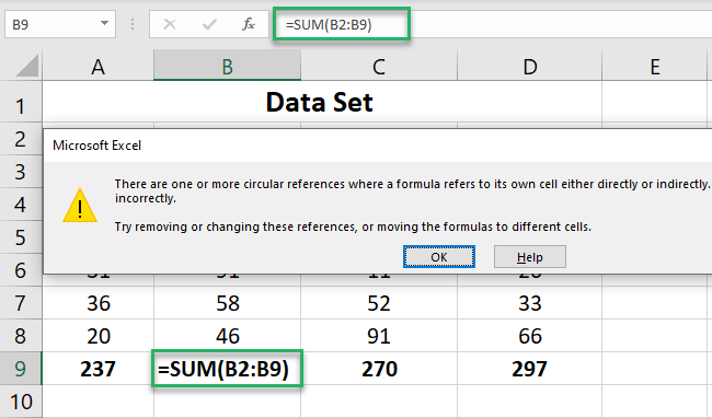
A circular reference error appears. This is because the formula SUM(B2:B9) refers to the same cell (Cell B9) where the formula itself is typed in.
If you click Ok, the SUM function will enter an endless loop and perform hundreds of calculations😵
It will then return an approximate result of the calculation i.e. zero – like this:
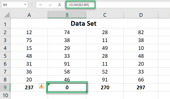
In this example, we exactly know where the circular reference exists for this formula (Cell B9).
But if you don’t know what causes the circular reference, you can still find it as follows:
- Go to the Formulas Tab > Formula Auditing.
- Click Error Checking.
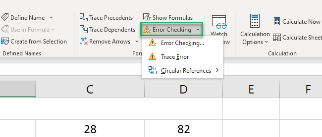
- Hover over Circular References.
Excel will show you the cell reference and even select it for you.

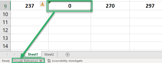
You can find the circular reference in the status bar as well.
If you still can’t find circular references in an Excel sheet, you can use trace arrows for help.
You can access them from the Formula Tab under the Formula Auditing group. These are represented by blue arrows.
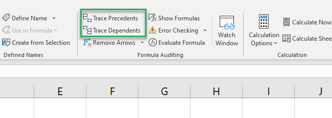
There are two types of arrows, namely:
- Trace Dependents
- Trace Precedents
Pro Tip!
Not in the mood to use your cursor? Not a problem – you can access these trace relationships using these sticky keys.
For Trace Dependents, use Alt + T > U > D;
And for Trace Precedents, use Alt + T > U > T.
Easy, no?
Trace Dependents point toward the cell whose value would be affected in case of change in that cell.

For example, the dependent for Cell B4 is Cell B9. If cell B4 changes, the value in Cell B9 (the sum of the row) would change too.
Trace Precedents show the cells that help you form the final result.

In our case, the Sum of cells B1:B8 results in the value in cell B9. So, the trace precedents for cell B9 are all the cells from Cell B2:B8 (and the blue arrow extends across them all).
How to fix a circular reference
Now that we know how to find a circular reference in Excel, let’s see how can you fix one🔧
Unfortunately, Excel has no defined method for removing circular references. This is why enabling circular references is not advised.
However, if you do want to remove circular references, you need to evaluate all the cells having circular references in Excel.
And then, you can manually alter the formula or write down a new one to fix a circular reference error✍
If your data is small, you might be able to easily spot the cell causing the circular reference and change it. Just like what we did here:
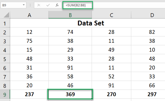
But if your data is a large one, you will have to find circular references using Error checking in Excel. And then eliminate the same manually.
You can also use trace arrows to help find the circular reference in Excel.
Disable circular references: Iterative calculations
Circular references are not enabled in Excel by default. And this is why Excel shows the error message prompt❗
However, you can enable iterative calculations if you want to use circular formulas in Excel.
Enabling iterative calculations tells Excel to run a calculation (or a formula) a certain number of times. This way Excel converges to a precise result.
But be warned❌ doing so is not recommended.
Nevertheless, to enable iterative calculation in Excel:
- Go to File > Options > Formulas.
- Put a checkmark in the Enable Iterative Calculation box under “Calculation Options”.

- If you want to disable it for some time, simply uncheck the box.
To further change the maximum iterations and maximum change :
- Go to Options > Formulas > Calculation options.
- Specify the desired value for both.
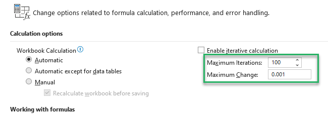
Maximum Iterations tell Excel how many times the formula is to be recalculated before the result is returned.
If even after the maximum iterations have been run, the formula criterion still isn’t met, Excel will stop calculating the result and return the final value as zero.
Remember how the result of the SUM function with a circular reference turned out zero in our example above💭
Maximum Change, on the other hand, measures the precision of the result. If you set it to 0.001, Excel will stop recalculating the formula when the difference between two possible iterations is less than 0.001.
That’s it – Now what?
In this article, we learned how to find and fix circular references in Excel. We also saw how to enable and disable Excel circular references.
It can be slightly challenging to locate the circular reference in Excel. Especially if you are dealing with a huge dataset.
But you can still find and fix it using the Error checking feature of Excel💪
Just like the error-checking feature of Excel, Excel functions are also of great use. Some of my favorite Excel functions include the VLOOKUP, IF, and SUMIF functions.
To get to know these (and more!) Excel functions, enroll in my 30-minute free email course now.
Other Resources
Did you enjoy reading this article? Seems like you are on the hunt for Excel errors and their solutions.
If so, do check out our other blogs on Excel errors. Like the #VALUE error, #REF Error, #NAME Error, and the IFERROR/ISERROR functions of Excel.
