How to Move Columns in Excel (6 Easy Methods)
Knowing how to move columns in Excel is as important as knowing how to copy and paste – it’s essential.
This is something you’d have to do almost all the time while you work in Excel.
So what are you waiting for?
Dive into the guide below where we have listed all the possible ways (and shortcuts) to move columns in Excel🚀
Also, to tag along with the guide, download our free sample workbook here.
Table of Contents
Method # 1: Using the Shift key
The first (and the basic) method of moving columns in Excel is by using the Shift key.
How? Look into the example below to understand that.
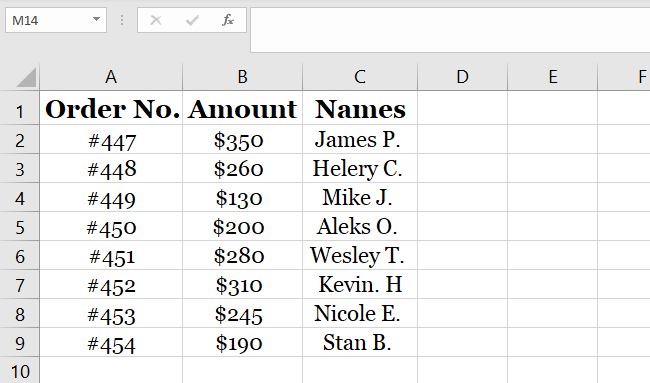
The data above consists of three columns.
Let’s say we want to move column C between Columns A and B. Here’s how we will do that:
- Select column C by clicking on the column header.
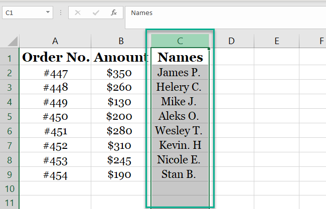
- Hover over the edge of the column and a plus sign appears.
- Hold down the Shift key when you see the plus sign.
- Drag the selected column to the targeted location (before Column B).
Pro Tip!
To move the columns in Excel while keeping the original data intact, we need to use the Shift command all along. This helps you move the columns to the targeted place without disturbing other data.
However, if you try to move the selected column as above using the Control Key, the targeted column will be replaced 🎯
The final result looks like this.
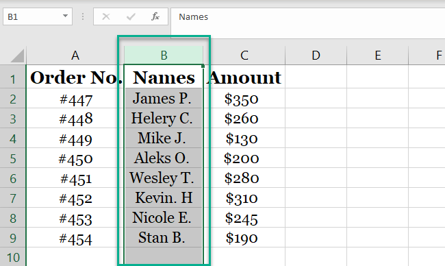
Column C (Names) is now placed between the column for Order Number and Amount.
Also, note how the column letter has automatically adjusted here (Column C is now Column B). You can do the same for rows in Excel.
If we had tried to do the same without using the Shift key, Excel would have shown a warning prompt 🚩
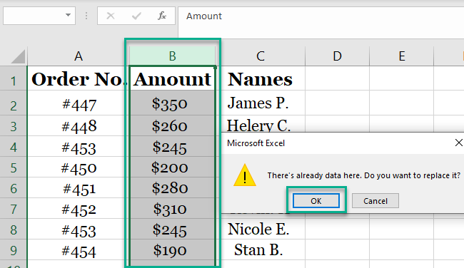
And the result would look something like this:
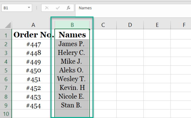
The original column B (Amount) is overwritten as we pasted column C in its place.
Method # 2: Using the insert, cut, and paste hack
This method is usually used by Excel newbies. And honestly, it’s not a very sophisticated approach for moving columns. Nevertheless, it works well.
The process is simple. You just select, insert, cut, paste, and delete. Bounced over your head?
Don’t worry – we’ve got a detailed explanation below.
Let’s use the same dataset as in the example above.
We again want to move column C between columns A and B, but this time, with a new method.
- Select the destined column (where you want to move Column C).
In our case, it’s column B (Amount).
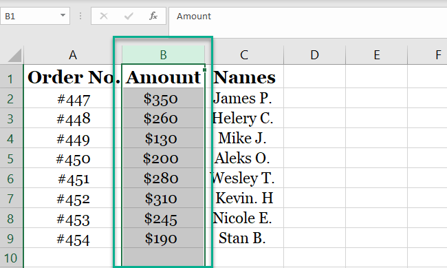
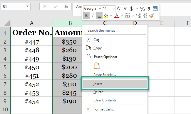
- Right-click column B and select the Insert option from the drop-down menu.
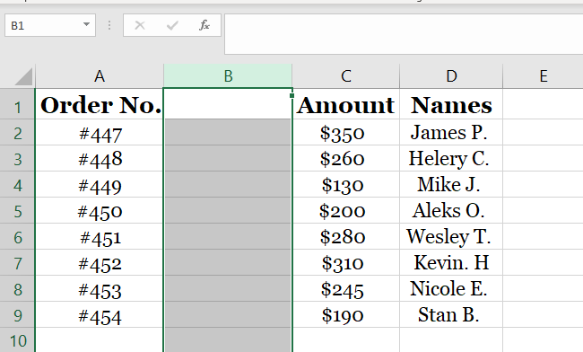
- A blank column will appear on the left side of the selected column:
- Select column D or press Ctrl + X to cut or CTRL + C to copy the entire column.
Note that after we’ve inserted an additional column before Column B, all columns have moved an alphabet ahead.
The column for Names (previously Column C) has now become Column D 👀
A moving, dotted enclosure will appear around the column. That’s when you’re ready to paste it to the new location.
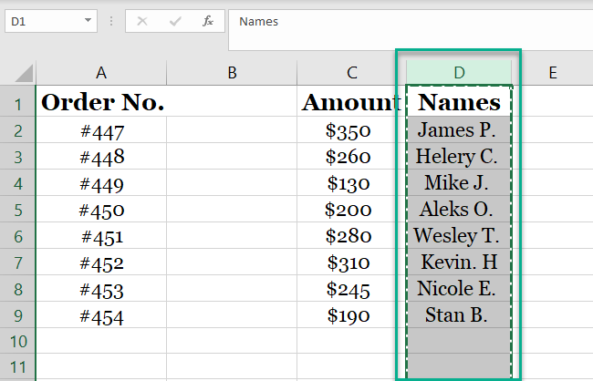
- Select the header Column B.
- Press down the Control Key + V to paste the column.
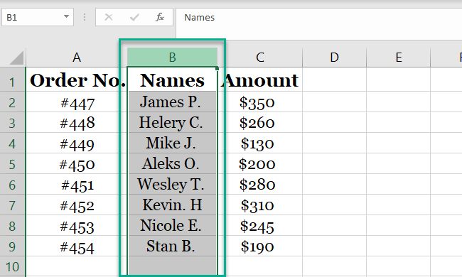
- Column D moves between columns A and C (previously Column B) successfully.
Too many steps and a little longer process? That is why this is not the best or the primary method to move columns in Excel.
Method #3: Using the CTRL key
Just like we can move columns using the Shift key, we can use the Control key for the same purpose too😍
There’s only one difference between both methods. When you copy columns using the CTRL key, the copied data is pasted into a new column. But, and that’s a big BUT – the data in the pasted column is replaced.
Didn’t get it? Let’s understand it through an example below.
We are using the same data as earlier, and we want to move Column C using the Control key this time.
- Select column C by right-clicking the Column C header.
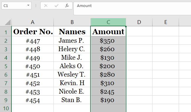
- Press down the Control key and hover over to the edge of the column until you see a plus sign.
- Hold and drag the column to the desired location.
- Column C replaces column B and appears right after the first column.
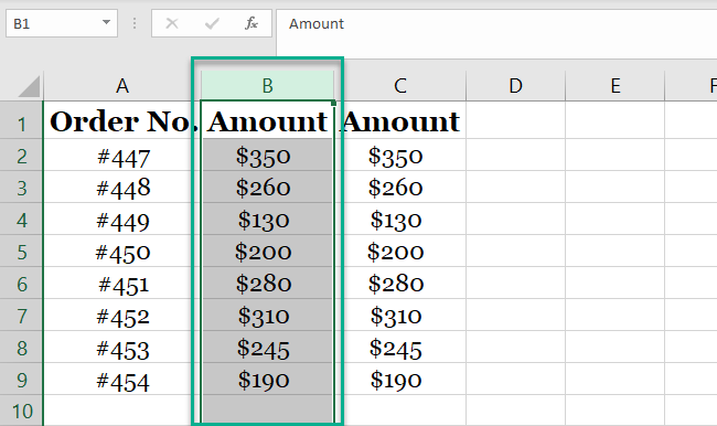
What happened here was that when we pressed the Control key, Excel made a copy of column C in place of column B by overwriting column B.
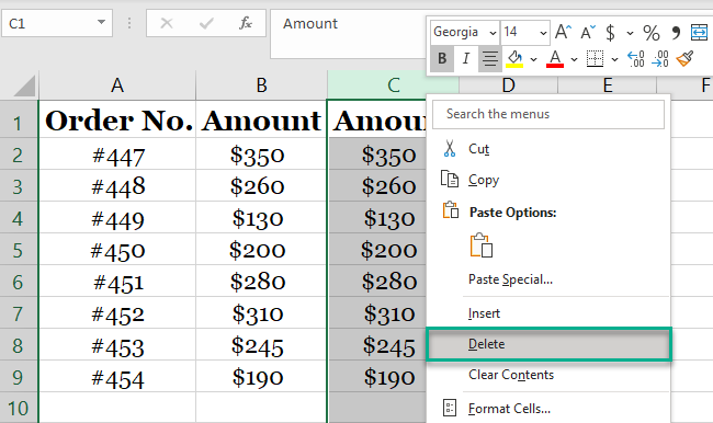
You can now delete column C by clicking delete from the context menu.
Method 4: Moving multiple columns at the same time
Okay, so now you know how to move a column in Excel. But do you know how to move multiple columns simultaneously?
We bet you don’t, and we’re here to teach you just that😎
Let’s say we have this dataset where we want to move columns B and C and bring them before column A.
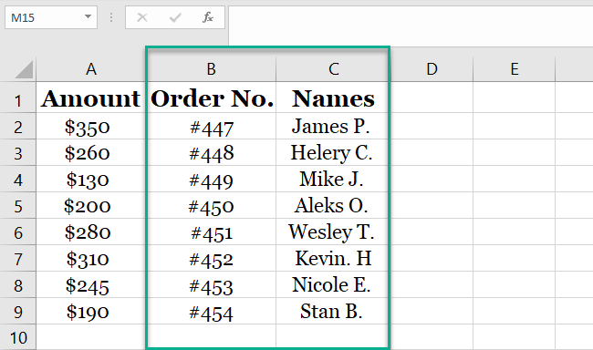
So, how do we do that? Using the Shift key method as we did previously.
- Select column C by clicking on the header.
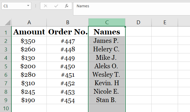
- Press down the Shift key and select the header for column B.
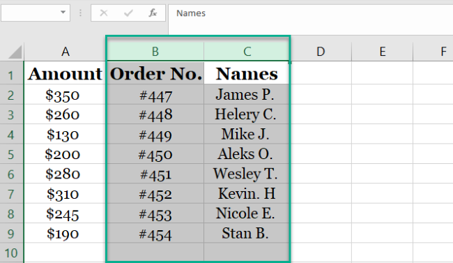
- Hover over the edge of Column B until the plus sign appears.
- Hold and drag the columns and drop them before column A.
- The result will look something like this:
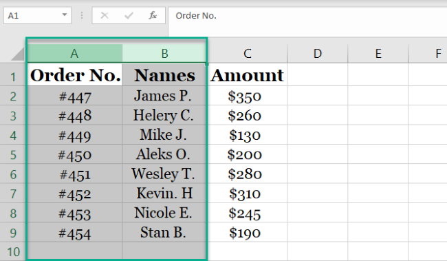
Note that this hack works for contiguous columns or contiguous rows only. You cannot use it to move non-contiguous rows and columns in Excel.
Method 5: Move columns to other worksheets
Now that we know how to work with columns in a single worksheet, it’s time we see how to move them to another sheet in the same workbook.
There’s a small but common hack for moving columns from one sheet to another. Let’s see it here👀
Using the same example as above, we are moving Column A from Sheet 1 to Sheet 3. To do so:
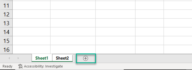
- Create a new sheet from the sheet tab at the bottom by clicking on the + sign shown below.
- Navigate back to Sheet 1.
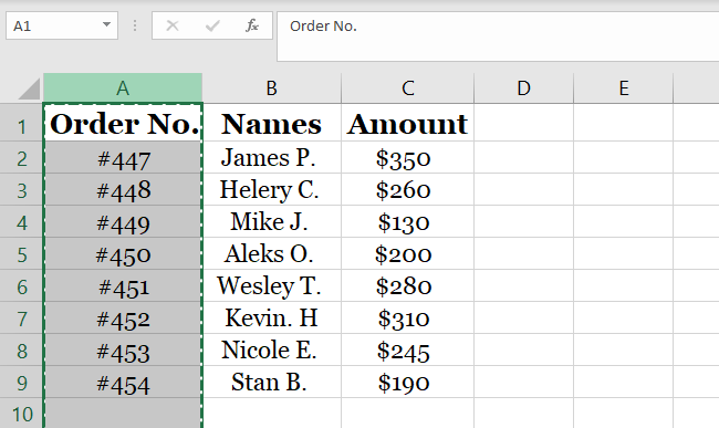
- Select column A and press CTRL + C if you want to keep a copy of the column in Sheet 1. Otherwise, press CTRL + X to cut the column.
- Go to Sheet 3.
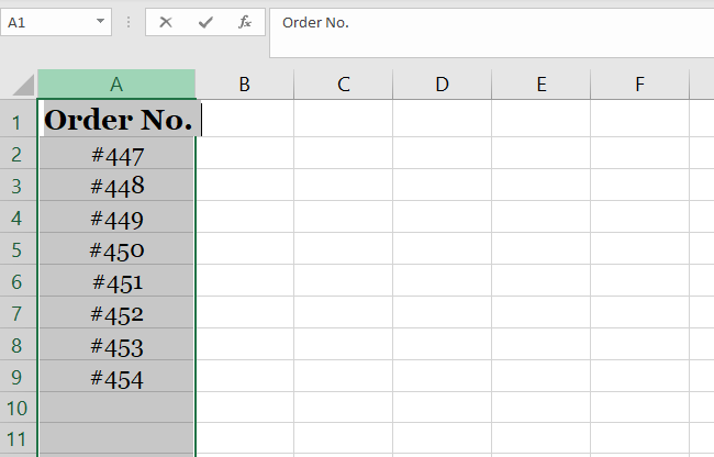
- Paste the contents in any column of Sheet 3 by selecting it and pressing CTRL + V.
For example, we’ve pasted it in Column A of Sheet 3 as shown below.
Method 6: Rearrange columns with horizontal sorting
You have probably heard about the Data Sort feature in Excel which allows you to sort your Excel tables. Usually, you vertically sort data in Excel.
But have you wondered if you can horizontally sort data too? 🤔
Yes, you can! More than that, you can use the Sort feature to rearrange your columns with horizontal sorting.
If you have a large spreadsheet and you want to change the order of numerous columns, horizontal sorting data could be a major time saver 👍
To start, you need to add a new row to the very top of your Excel spreadsheet. So…
- Right-click row header 1.
- Select Insert from the right-click menu.
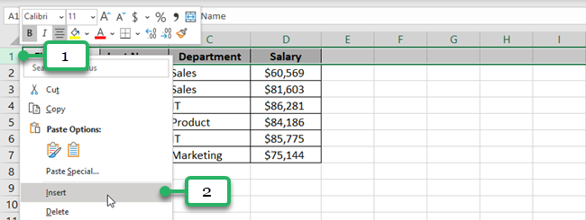
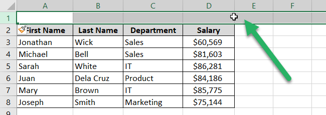
A new row is inserted in your worksheet.
This row must be at the top of the page, above all other header rows or labels.
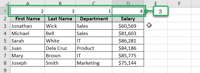
- Number the existing columns in the order you want them to appear in the spreadsheet. Enter the numbers in the new top row.
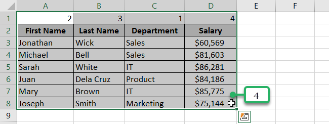
- Select all the data in the table that you want to rearrange.
- Go to the Data Tab.
- In the Sort & Filter Group, click Sort.
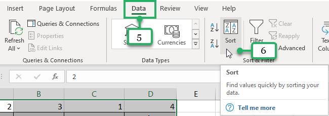
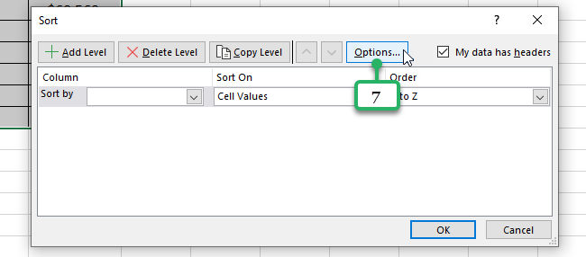
The Sort Dialog box appears on your screen.
- Click the Options button.
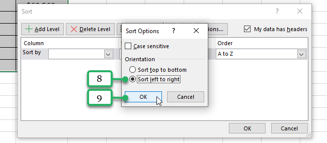
- Select Sort left to right.
- Click OK.
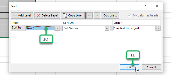
This returns you to the Sort dialog box.
- In the Sort By drop-down menu, select Row 1.
- Finally, click OK.
This is now the result ✅
The columns are now rearranged according to the order in which you wanted them to appear.
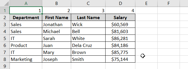
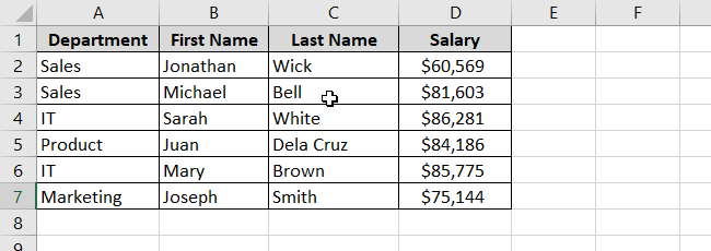
Now that the columns are rearranged, you can delete the very first row.
And voila! 😀
When moving columns, Excel copies the content in cells and moves them to the new location you want them.
This includes text values, numeric values, formulas, and cell formats.
However, cell references are not adjusted. You need to manually adjust the column references. If not, you may see a #REF! error in your cells. So, be careful!
That’s it – Now what?
In this article, you’ve learned the 6 ways to move columns in Excel – this should accommodate any situation you encounter🔰
But there is so much more you can do with columns in Excel. And this article doesn’t do justice in covering even 5% of that information.
There are tons of other things to Excel that you’d want to learn. You can start by practicing with core Excel functions like the VLOOKUP, IF, and SUMIF functions.
Enroll in my 30-minute free email course today to learn these functions (and more!).
Other resources
Want to organize your data better? Check out our guide on how to sort in Excel to transform your spreadsheets.
Want to flip your Excel table from rows to columns? Follow our step-by-step tutorial on transposing data. 😊
