15 Most Common Excel Functions You Must Know + How to Use Them

Microsoft Excel is one of the most well-known computer applications. It has changed the way people and companies work with data.

Thus, learning Excel can help with both your career and your personal needs.

Excel runs using functions and there are roughly 500 of them! These range from basic arithmetic to complex statistics.

If you’re a new Excel user, this sheer quantity can be quite daunting.

So we are here to help you! 🤝

We have rounded up 15 of the most common and useful Excel functions that you need to learn. We also prepared a practice workbook for you to follow along with the examples. Download it here.

Let’s get started!

What are Excel functions?

Excel is used to calculate and manipulate numbers and text. To do this, you use formulas!

Formulas are expressions that tell Excel what you want to do with the data. They begin with the equal symbol (=) followed by a combination of operators and functions.

What are operators?

These are symbols that specify the type of calculation you want to perform on the elements of a formula.

For example, to add two numbers, you can type “=1+1” into a cell. Once you hit Enter, Excel will run the formula and return the result which is 2.

Here are some examples of common operators:

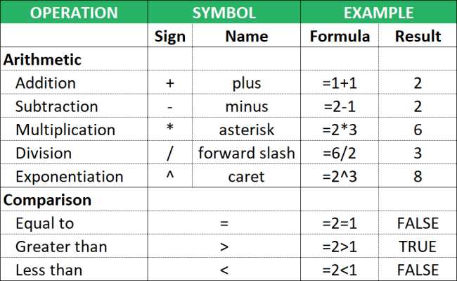
Excel automatically treats cell contents that start with (=) as formulas. This also applies when you begin a cell with the plus (+) or minus (-) symbols.

You can bypass this by adding a leading apostrophe (‘). This is how you can show formulas as text like in the table above.

Order of operation and using parentheses in Excel formulas

Generally, Excel follows PEMDAS when calculating formulas. PEMDAS means parentheses first, then exponents, then multiplication and division, then addition and subtraction.

What are functions?

These are predefined processes in Excel. Each function in Excel has a unique name and specific input(s). The function takes these inputs and performs the corresponding calculation.

The inputs or arguments of an Excel function are always enclosed in parentheses.

For example, this is the syntax for the MAX function:

=MAX(number1, [number2], …)

The list of numbers where you want to find the maximum value is placed inside the parentheses.

Using a cell or a range as input

As you learn more about Excel, you’ll find that Excel formulas rarely consist of individual numbers only like in the formula “=1+1”.

Thus, referencing cells is important in Excel and you can learn more by clicking here.

Alright! You’ve just learned how a function in Excel works.

Let’s dive right into the list! 🤿

We will start with basic Excel functions and then move on to more advanced functions.

Basic Math Functions (Beginner Level ★☆☆)

1. SUM

This is the first function in Excel that most new users need. As the name implies, the SUM function adds up all the values in a specified group of cells or range.

Syntax: =SUM(number1, [number2], …)

Try it out in the practice workbook.

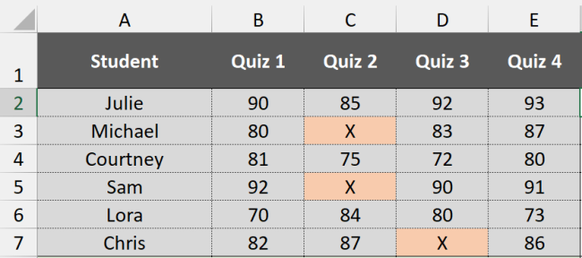
If you want to get the total quiz score for each student, you can use the SUM function. In this case, the input range will be all four quiz scores for each student.

1. Type this formula into cell F2:

=SUM(B2:E2)

You can also type “=SUM(B2,C2,D2,E2)” but “=SUM(B2:E2)” is much simpler.

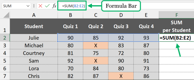
2. Press Enter. Excel then evaluates the formula and the cell returns the number for the total which is 360.

3. Copy this for the rest of the students or drag down the fill handle.

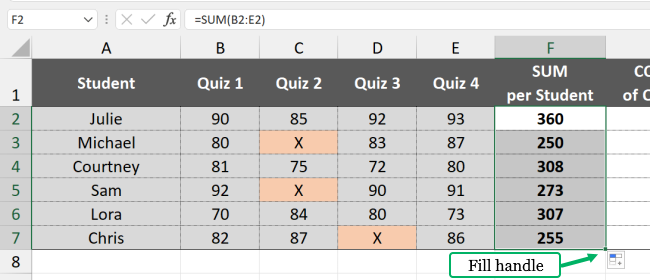
Notice that the SUM function ignores the cells containing text. (“X” meaning the student was unable to take the quiz)

Most of the basic math functions in Excel ignore non-numeric values such as text, date, and time.

2. COUNT

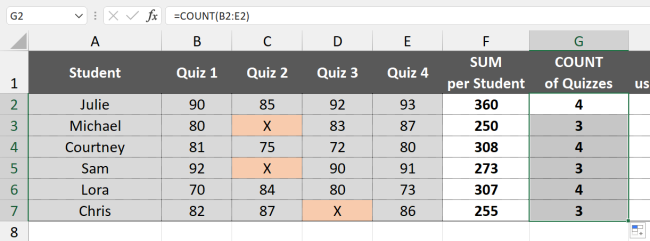
Next up is the COUNT function. It returns the number of cells containing numeric values within the input range.

Syntax: =COUNT(value1, [value2], …)

1. To get the number of quizzes taken by each student, use this formula in cell G2:

=COUNT(B2:E2)

2. Hit Enter and fill in the rows below.

If you would like to include non-numeric values in the count, you can use the COUNTA function. To count the number of blank cells, you can use the COUNTBLANK function.

Learn more about the COUNT function and its variants here.

3. AVERAGE

The average of a list of numbers is just the total divided by how many numbers there are in that list.

This is easy enough to calculate the quiz scores. You already have the SUM and the COUNT of quizzes for each student.

But, it gets even easier using the AVERAGE function in Excel.

Syntax: =AVERAGE (value1, [value2], …)

1. Type this into cell H2:

=AVERAGE(B2:E2)

2. Hit Enter and fill in the rows below.

The AVERAGE function also has variants for more advanced calculations. Click here to learn more.

Logical Functions (Intermediate Level – ★★☆)

Let’s raise the difficulty level a little bit.

A logical function in Excel allows you to make comparisons and use the results to change how a formula calculates.

4. IF

The IF function is a very popular function in Excel and it is actually quite easy to learn.

Syntax: =IF(logical_test, value_if_true, [value_if_false])

This function checks if a logical test is either TRUE or FALSE. It then returns the specified value based on the result.

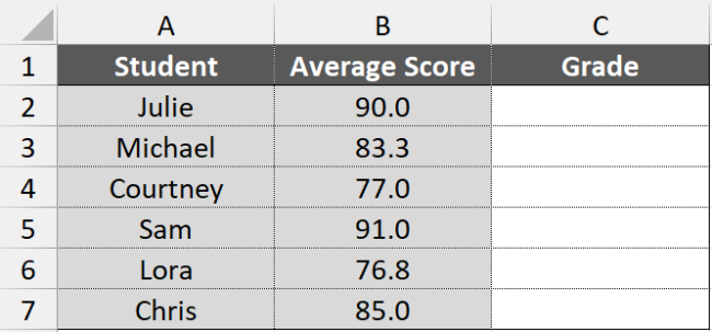
Using the average score of each student, try to assign PASS or FAIL grades. Assume that the passing score for this class is 60.

1. Begin the formula in cell C2 with “=IF(“

The logical_test is to check if the average score in Column B is greater than or equal to (>=) the passing score of 60.

2. So, the formula becomes:

=IF(B2>=60,

If the comparison returns TRUE, then the formula should return the text “PASS”. Thus, the value_if_true argument should be “PASS”.

And if it returns FALSE, then the value_if_false argument should be “FAIL”.

3. Thus, the formula becomes:

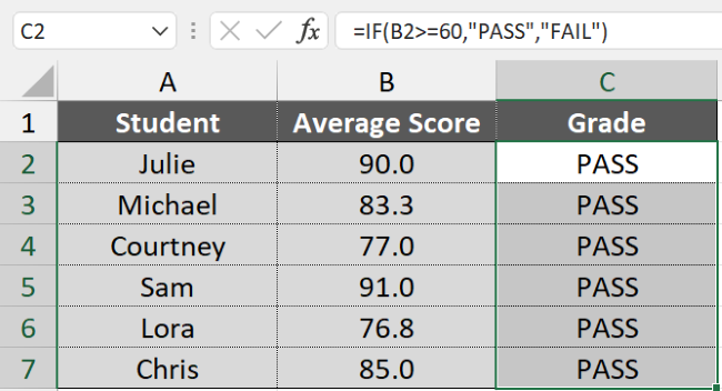
=IF(B2>=60,”PASS”,”FAIL”)

4. Hit Enter and fill in the rows below.

What if you needed to assign grades according to a scale instead of just “PASS” and “FAIL”?

For that, you have to use multiple criteria or logical tests. While this is possible using nested IF functions, it can get messy very quickly. Instead, you can use the IFS function.

5. IFS function

The IFS function was introduced in Excel 2016 to replace nested IF functions.

This function works by evaluating the first logical test or criteria. It returns the corresponding value if it is TRUE. But if it is FALSE, the function proceeds to evaluate the second criteria, and so on.

📖 In other words, the IFS function outputs the value that corresponds to the first specified criteria that is true.

Syntax: =IFS(logical_test1, value_if_true1, [logical_test2], [value_if_true2],..)

1. First, the formula should check if the average score (column B) is above or equal to 90. If yes, it should return “A”.

=IFS(B2>=90,”A”,

2. If not, it should then check if the average score is greater than or equal to 80. If yes, it should return “B”. If you do this up to grade D, the formula becomes:

=IFS(B2>=90,”A”,B2>=80,”B”,B2>=70,”C”,B2>=60,”D”,

3. For the last grade “F”, put “TRUE” for the logical test.

The IFS function will only evaluate the last specified criteria if all of the previous logical values were FALSE. Thus, you can set the last criteria to always be TRUE thus making it a “catch all” statement.

The final formula is then:

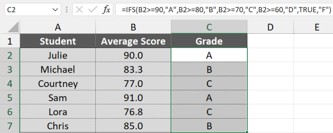
=IFS(B2>=90,”A”,B2>=80,”B”,B2>=70,”C”,B2>=60,”D”,TRUE,”F”)

PRO-TIP:

You can use absolute cell references and a reference table when working with long formulas.

That way, you don’t have to revisit all of the arguments in the formula if you need to change some values.

For example, using the table and formula shown below, you can easily change the grading scale in use.

=IFS(B2>=$H$2,$F$2,B2>=$H$3,$F$3,B2>
=$H$4,$F$4,B2>=$H$5,$F$5,TRUE,$F$6)

Text Functions (Intermediate Level – ★★☆)

In this next section, you will see how Excel can also be used to manipulate text.

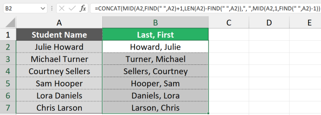
In the “Class List” worksheet of the practice workbook, the full name of each student is listed in Column A. Your goal is to rearrange these from “first name last name” to “last name_first name” in Column F.

To do this, you first have to extract the first name and the last name from Column A.

6. FIND

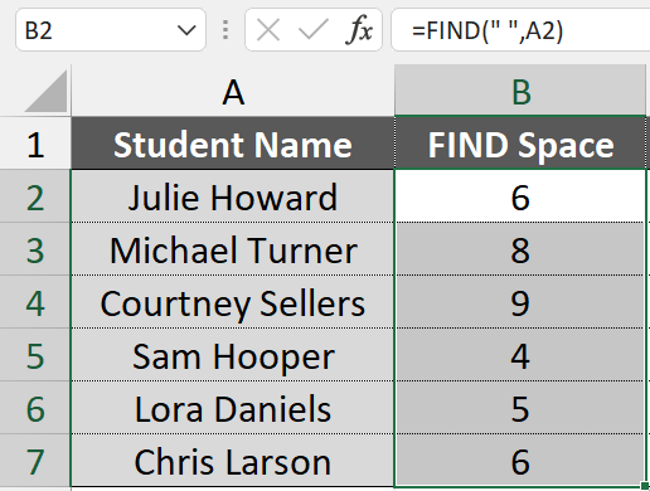
The names are separated by a space character ” “. So, you have to identify the position of the space within each text string in Column A.

The FIND function in Excel returns the number or position of a specified character or substring within another text string.

Syntax: =FIND(find_text, within_text, [start_num])

To get the position of the space ” “, type this formula:

=FIND(” “,A2)

Next, take a look at the LEN function.

7. LEN

This function returns the number of characters in a text string.

Syntax: =LEN(text)

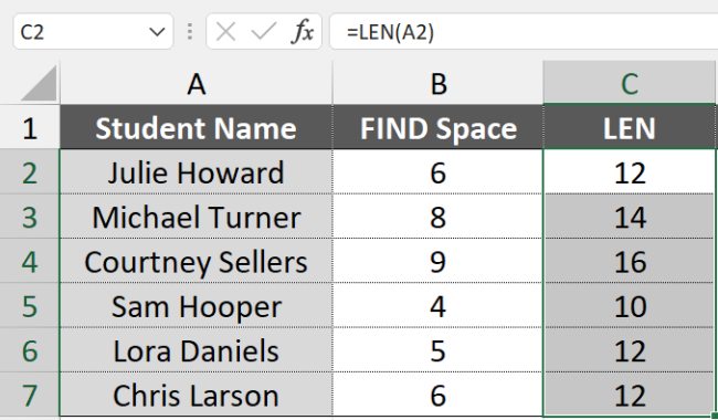
To get the number of characters in each student’s name:

=LEN(A2)

Now you can move on to extracting the first and last name using the MID function in Excel.

8. MID

This function extracts a given number of characters from the middle of a text string.

Syntax: = MID(text, start_num, num_chars)

It is one of three text functions that are used to extract text. The other two are LEFT and RIGHT which extract text from the start and end of a text string respectively.

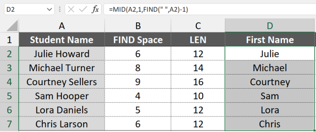
The first name starts at the very first character of the text string. So, you extract starting from position 1. Then the length of the first name is given by the position of the space character minus 1.

So, the formula to extract the first name or first word from a text string is:

=MID(A2,1,B2-1)

Or, you can express it directly using the FIND formula earlier.

=MID(A2,1,FIND(” “,A2)-1)

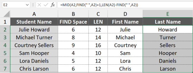
For the last name, you can extract it starting from the position of the space character plus 1. Its length is just the length of the entire text string minus the position of the space character.

=MID(A2,B2+1,C2-B2)

Or, using the FIND and LEN formulas earlier:

=MID(A2,FIND(” “,A2)+1,LEN(A2)-FIND(” “,A2))

Now you can combine the last name and the first name in the desired order using the CONCAT function.

9. CONCAT

Like IFS, CONCAT is another newly introduced function in Excel 2016. It replaced the old CONCATENATE function.

Syntax: =CONCAT(text1, [text2],…)

Combine the last name and the first name with a comma and space character “, ” in between.

=CONCAT(E2,”, “,D2)

PRO-TIP:

In the above example, you used helper columns for FIND, LEN, and MID to help build the final formula and visualize how it works.

In real-world applications, you can use a single long formula to get the results like this:

=CONCAT(MID(A2,FIND(” “,A2)+1,LEN(A2)
-FIND(” “,A2)),”, “,MID(A2,1,FIND(” “,A2)-1))

Lookup and Reference Functions (Advanced Level – ★★★)

In this final section, we will focus on functions that allow you to look for specific data points and refer to them.

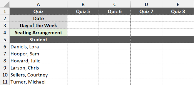
Take a look at the “Schedule” worksheet.

10. COLUMN

The COLUMN function in Excel returns the column number of a given cell.

Syntax: =COLUMN([reference])

Let’s try to assign specific dates for each quiz. For example, you may want the quizzes to be held every Monday. This means that the first quiz date should be offset by 1 week or 7 days for each succeeding quiz date.

You can use the column number to multiply the 7 days offset for each week like this:

=$B$2+(COLUMN()-2)*7

Two (2) is subtracted from the column number so that the sequence starts at 1.

You can also get this result using the much simpler “=B2+7” since you are only adding a fixed number of days to each date. 🤔

But, using the COLUMN function, you can create complex patterns.

Take this pattern for example:

The quizzes are still held every Monday. But every third week, they are held on Wednesday instead.

Here is the formula for this pattern:

=$B$2+(COLUMN()-2)*7+IF(MOD(COLUMN()-1,3)=0,2,0)

11. ROW

Next, take a look at the ROW function. It works exactly like COLUMN but it returns the row number instead.

Syntax: =ROW([reference])

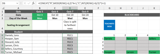
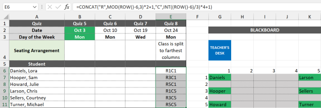
In this next example, you will assign the seating plans. You can try different seating arrangements using the ROW function.

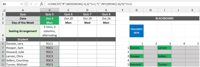
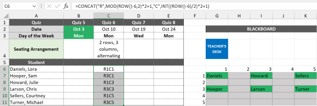
Assume R1C1 is the seat closest to the teacher’s desk.

1. You can have the students seated one seat after another and in two columns:

=CONCAT(“R”,MOD(ROW()-6,3)*2+1,”C”,INT((ROW()-6)/3)*2+1)

2. Or they can sit in rows of 3 and columns of 2

=CONCAT(“R”,MOD(ROW()-6,2)*2+1,”C”,INT((ROW()-6)/2)*2+1)

3. You can also sit them in the farthest rows:

=CONCAT(“R”,MOD(ROW()-6,2)*4+1,”C”,INT((ROW()-6)/2)*2+1)

4. Or in the farthest columns:

=CONCAT(“R”,MOD(ROW()-6,3)*2+1,”C”,INT((ROW()-6)/3)*4+1)

Manually creating seating patterns for small sets like this one is easy. But a formula like those shown above definitely helps especially for larger sets like 50, 100, or even more.

The COLUMN and ROW functions are rarely used on their own. Like IF and IFS, you use them with other functions to change how the formula is calculated.

12. MATCH

Now, open up the “Lookup” worksheet.

In the next few examples, you will create a search feature that allows students to look up their names. They can then see their scores from past quizzes and their assigned seats for the next quizzes.

To start, you will use the MATCH function. It searches for a specified item within a given range of cells. It then returns the relative position of the first match.

Syntax: =MATCH(lookup_value, lookup_array, [match_type])

1. The lookup_value is the item you want to search for. So, set this to cell B2.
2. The lookup_array is the range or table array where you want to search. Use F2:F7 from the “Class List” worksheet.
3. For the match_type, set this to zero so that the function searches for an exact match. (Learn more about MATCH and the different match types in this article)

The formula then becomes:

=MATCH(B2,’Class List’!F2:F7,0)

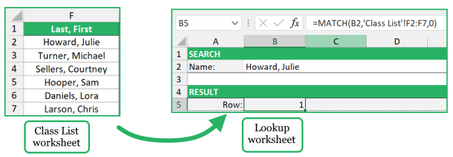
However, it only works correctly if the name is entered exactly as it is written in Column F of the Class List.

To fix this, you can use the asterisk “*” wildcard character so that searching for either first or last name works.

You can also enclose the formula in an IFNA function. This way, if the formula cannot find the given name in the table, it will return a phrase like “No result found”.

13. INDEX

The INDEX function retrieves a value from a given table array based on the provided row and column numbers.

Syntax: =INDEX (array, row_num, [col_num])

Similar to the MATCH example, you need to specify where the range or array lookup is.

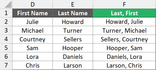
For row_num, you can use the earlier MATCH result at Cell B5. Then for col_num, use 1 for the First Name:

=INDEX(‘Class List’!D2:E7,B5,1)

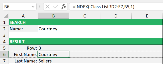
And set col_num to 2 for the Last Name.

=INDEX(‘Class List’!D2:E7,B5,2)

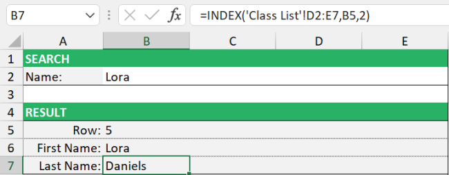
Just like that, you have a working search 🔍 formula!

This is just a small example of the countless possibilities using the INDEX and MATCH combination. Click here for more examples!

14. VLOOKUP

The VLOOKUP function in Excel works similarly to the INDEX and MATCH combination. It is faster to set up but it is less versatile. VLOOKUP also only works if your lookup array is at the leftmost of the reference table.

Syntax: =VLOOKUP (lookup_value, table_array, col_index_num, [range_lookup])

This time, you will use the First Name result (cell B6) as the lookup_value. Use this and VLOOKUP to retrieve the given student’s scores from the “Quiz Scores” worksheet.

=VLOOKUP($B$6,’Quiz Scores’!$A$2:$E$7,COLUMN(),FALSE)

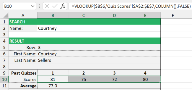
For the seat assignment, use the Last Name result followed by the asterisk wild character.

=VLOOKUP($B$7&”*”,Schedule!$A$6:$E$11,COLUMN(),FALSE)

15. INDIRECT

The last function that you will be learning about today is also one of the most powerful in Excel.

INDIRECT allows you to specify cell references using text strings.

SYNTAX: =INDIRECT(ref_text, [a1])

For example, instead of typing “=A1”, you can type “=INDIRECT(“A”&1). This means you can dynamically change references.

Let’s take the INDEX & MATCH formula you used to retrieve the Last Name. You can get the same result using this formula:

=INDIRECT(“‘Class List’!”&”E”&(B5+1))

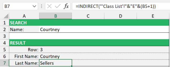
The INDIRECT function opens up so many possibilities with dynamic references in Excel. I highly this article for an in-depth tutorial on INDIRECT.

That’s it – Now what?

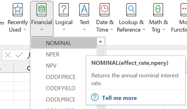
As you have just learned, Excel offers so many different functions to choose from. Luckily, Excel has brought them all together in the Formulas tab.

You can look for an Excel function using search keywords or you can also select from the categorical dropdowns.

For example, click on the Financial group to find functions that can help you calculate items like net present value, future value, cumulative interest paid, cumulative principal paid, etc.

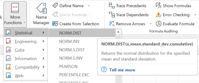
You can also click on More Functions which opens up even more possibilities for advanced Excel formulas.

For example, the Statistical group is useful if you need to calculate a statistical value. This includes functions for maximum value, minimum value, forecast value, gamma function value, etc. You can insert a cumulative distribution function and other useful tools for data analysis.

Learn how to use these formulas and more by signing up for my free online Excel course.

We will help you make the most out of your Excel experience! 📈

Other relevant resources

If you enjoyed this article, you can visit my YouTube channel for more in-depth tutorials and other fun stuff!

Did you know that the Flash Fill feature can help speed up your work by automatically filling a repetitive pattern Excel detects from your data? Learn more here.

Thanks for reading! 😄