Full List of ALL Excel Errors and How to Fix Them
Hashtags are a trend – yes, but only until they are on Instagram or maybe Twitter. As soon as you see your Excel sheet throwing hashtags your way, you know there’s something wrong 🛑
Excel errors come with a hashtag before them #️⃣
Like the #DIV/0 error, #NAME? Error and so on. And there’s always some specific reason why you’d see these errors in Excel.
Learn about that reason and remove it to fix the errors in your Excel sheet through the guide below. We have them all (the Excel errors) sorted for you here.
So glide in and download our free sample workbook on your way to tag along with the guide 📩
Table of Contents
#DIV/0 error
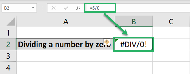
The #DIV/0 error tells that you are dividing a number by zero. And let me take you back to Grade 6, where we learned that a number divided by zero is undefined 👩🏫
Practically, no number is divisible by zero. And that is why if you try dividing a number by zero in Excel, you end up with a #DIV/0 error.
For example, check this out:
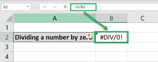
Similarly, if you divide a number by a blank cell, here’s what you get.
Also, if you have a #DIV/0 error in a cell and you refer to it in any other formula, you’d still get the #DIV/0 error.
For example, here we’ve referred to Cell A2 (that contains the #DIV/0 error) in our formula =A1+A2+A3, and this is what we get 🤦♀️
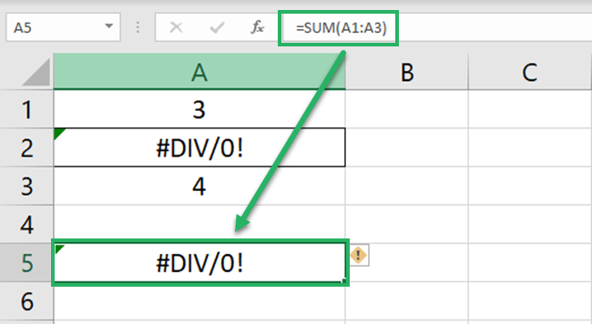
The answer is again a #DIV/0 error.
Some quick ways how you can prevent the #DIV/0 error in Excel include ensuring the following:
- Your formulas do not refer to any cells containing the #DIV/0 error
- You don’t perform the division operation using any empty cells.
- The cells in your dataset do not contain zeros
In addition to these, you can also use the IFERROR function to replace the #DIV/0 error in your worksheet with any other value as desired 👌
How? Learn more details about it by reading our tutorial on the #DIV/0 error here!
#N/A error
In simple words, the #N/A error means that the underlying formula failed to find what it had been told to find.
For example, if you write the VLOOKUP function to find the sales of “P” from the data in the image below:
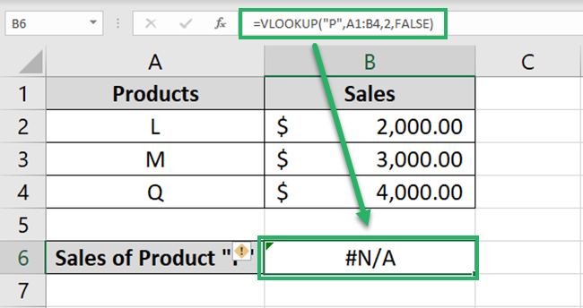
You’ll get the #N/A error because there is no “P” in the data above. And the VLOOKUP function is set to find the data under the exact match mode.
It fails to find the given lookup value – and we end up with a #N/A error ❌
The function might not be able to find the given value for several reasons. Maybe because it’s not in the right format, or maybe because the spelling of the look-up value doesn’t match.
You’d most likely see the #N/A error in Excel when you’re using the lookup functions i.e. VLOOKUP, HLOOKUP, MATCH, etc.
You can prevent (or fix) the #N/A error by trying the following:
- The lookup value is correctly spelled. No special characters or extra spaces to it.
- The lookup table contains the lookup values.
- The match mode (exact or approximate) is in line with the look-up value.
#NAME? error
As the name suggests, the #NAME error occurs when you have misspelled a name. It could be the name of a function, the name of a named range, or even an incorrect argument.
For example, check out here 👀
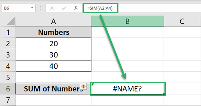
If you misspell the SUM function as the SIM function, you get the #NAME error.
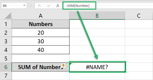
Similarly, if you have saved a range by a name in Excel, misspelling it will cause the #NAME error as below.
Here the name of the range was “Numbers” and we misspelled it as “Number” 🔢
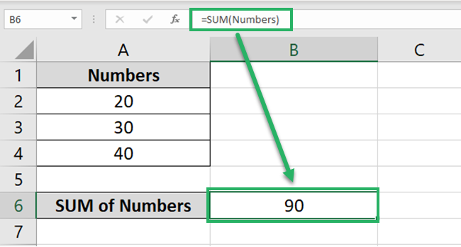
When the range is rightly spelled as “Numbers”, the results change as follows:
To avoid this problem, type in the first letter of the formula and press the “Tab” key.
Excel will enter the name of the function for you so there is no more chance of spelling mistakes.
And yeah! You’d also get the #NAME error if you wrongly write the reference for a range. Like we have forgotten the colon between A2 and A4 (A2A4 instead of A2:A4) here. So we get the #NAME? error 📍
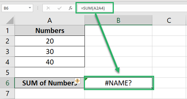
Be careful with the spelling and you’d most likely avoid the #NAME Error in Excel. Learn more reasons why the #NAME error occurs in Excel and how can you fix it here.
#REF! error
The #REF error is Excel’s way of saying that there’s something wrong with the cell references in your formula.
For example, if you write a function with some cell references (say A2, A3, and A4).
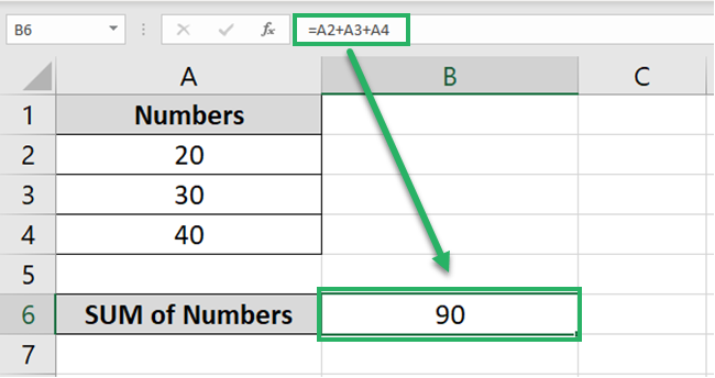
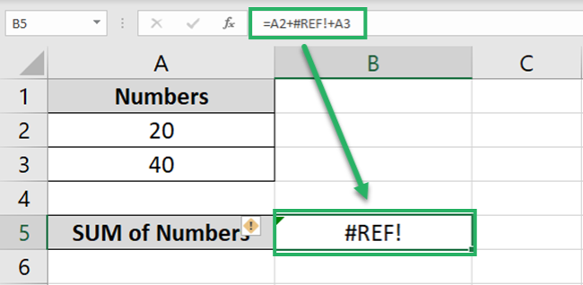
And then delete a row (say Row 3), and you’d get the #Ref! error as below 👎
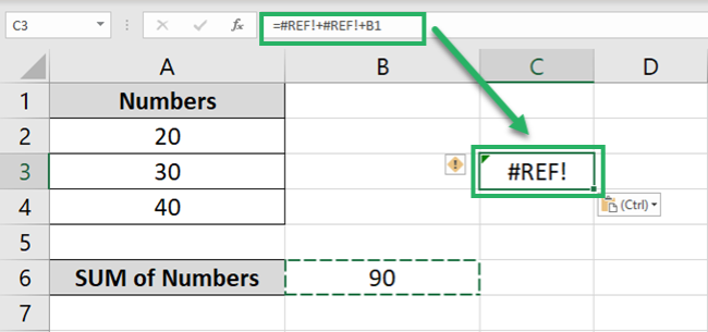
#REF! error also occurs when you copy-paste formulas that contain relative references from one cell to another.
Like here we copied the formula =A2+A3+A4 from one cell to another, and this is what we get.
Some ways how you can avoid the #REF errors in Microsoft Excel include the following 🤩
- Don’t delete the structural part of any row, column, or sheet unless abundant.
- Use in-built functions of Excel and not operations.
- Turn your references into absolute references before you copy/paste formulas.
There are much more details to the #REF error of Excel – what causes it and how it is fixed. Learn all about it here.
#VALUE! error
You’d see the #VALUE error popping up in your Excel sheet when there is something wrong:
- With how the formula is typed.
- Or with the cell references in your formula.
For example, here we have specified the wrong data type for the PRODUCT function:
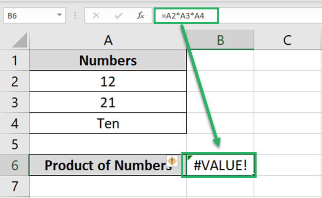
Excel can surely multiply numbers but not text. As the list contains the text “ten”, the formula to add them up returns a #VALUE error ✖
Similarly, if you write arguments for a function that don’t make sense, you’d again see the logical error.
For example, the FIND function of Excel finds the position of a character from a text string.
The formula FIND (“p”, “paint”) gives the result 1. Because the substring “1” comes in the second position in the word “paint” 🎨
Try writing this formula as below:
=FIND (“b”, “kite”)

And Excel returns a #VALUE error. Because the word “kite” just doesn’t contain the character “b”, let alone its position therein 🪁
The exact reasons why the #VALUE error may occur depending upon the formula being used. However, the following general hacks can help you fix it.
- Double-check the format of your data. For example, if it’s a date function, make sure the arguments you enter are in the date format.
- Use Excel’s in-built functions instead of writing formulas yourself.
- Look out for any special characters in cells that may make your formula invalid.
####### error
It might be a little unfair to call this an error. If you are an Excel user, you must have come across a series of hashes in your spreadsheet in Excel that looks like this:
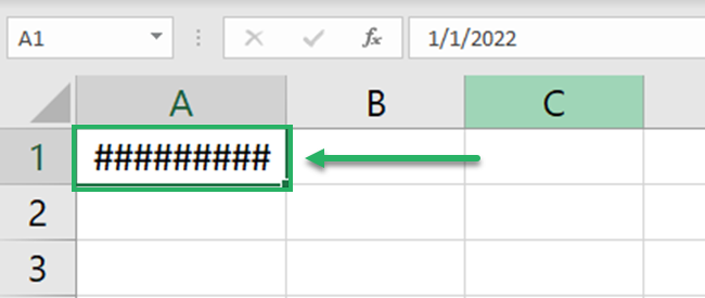
Well, that’s not a reason to worry #️⃣
This simply means that the column width for the subject cell is not enough to contain the value you’re trying to fit in.
So how can you fix this? Need not ask. Simply resize the column to broaden its width. To do that:
- Hover your cursor over the column header until a double-headed arrow appears.
- Once you see it, double-click it, and Excel would automatically resize the column to fit the value.
Alternatively, to autofit the width of your column:
- Go to the Home tab > Format > AutoFit Column Width
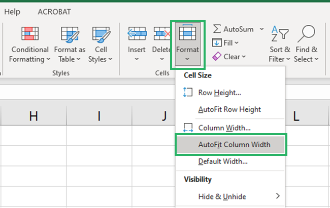
And as a last resort, you can also broaden a column manually until it is wide enough to contain the given value (you’ll get to know that when the hashes are replaced by the value).
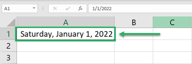
For example, here we resized the column, and the hashes are no more there 🔧
#NULL! Error
I’d not be surprised if you told me you’d never seen this error in Excel before. The #NULL! Is not very common 🤨
It occurs when a space character replaces any of the following:
- The colon between two cell references (like A2 B2 instead of A2:B2)
- The comma between two arguments.
And as you replace the space character with the relevant character (a colon or a comma), the error goes away 💪
For example, in the image below, we have written the SUM function as follows:
= SUM (A2 A3)
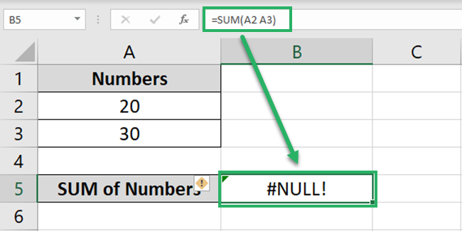
Note that instead of a comma between both arguments, there is a space character 🏹
The SUM function throws a #NULL error our way. Rewrite the SUM function by replacing the space character with a comma.
= SUM (A2,A3)
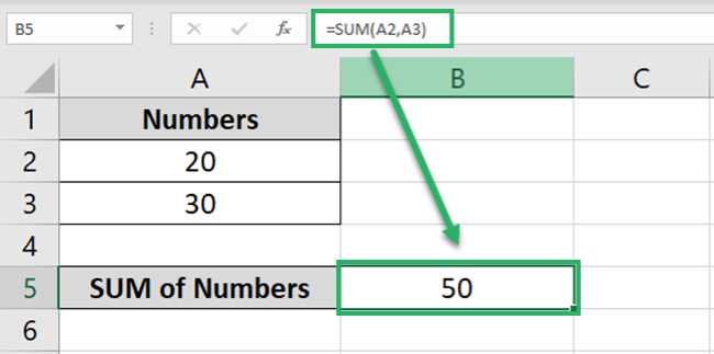
And suddenly, everything’s fixed in place 😍
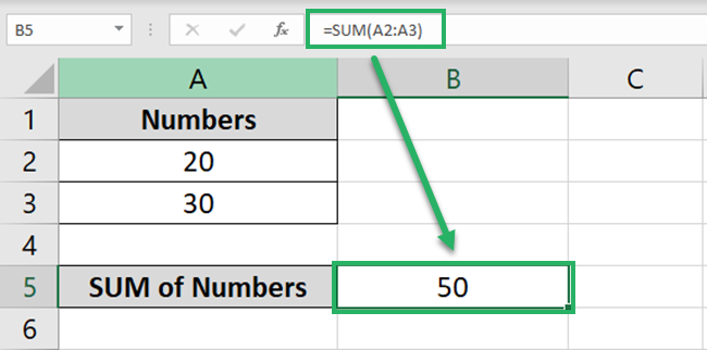
Similarly, if you had replaced the space character with a colon, this would have been the result:
= SUM (A2:A3)
#SPILL error
The #SPILL error appears in Excel when the spill range is not empty to contain the results of any formula.
#SPILL error only comes for formulas whose results extend beyond the boundary of a single cell. For example, if you write an array formula like this:
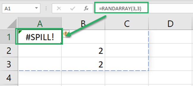
You end up having a #SPILL error 🙈
But why?
The RANDARRAY function returns an array of random numbers. In our example above, we wrote the formula to get an array of 3 rows and 3 columns.
But note that column 2 and row 2 were not vacant – they had some values. And as the spill range was not empty, RANDARRAY failed to populate them with the array of random numbers.
That’s how you end up with a #SPILL error.
Remove these values from the spill range and reapply the RANDARRAY function to see how the results change.
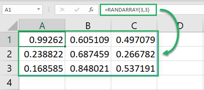
The #SPILL error also occurs if you apply a dynamic array function to an Excel table. Dynamic array functions are not supported by Excel tables 🙅♂️
The #SPILL error comes with formulas that produce an array of results. And so, you’ll mostly see the #SPILL error in newer versions of Excel that support dynamic array functions.
Here are some quick ways to fix the #SPILL error in Excel ⛏
- Ensure your spill range is vacant to contain the array of results.
- Ensure none of the cells of your spill range are merged.
- Don’t use dynamic array functions with Excel tables.
#CALC!
The #CALC error occurs when a dynamic array function runs into a calculation error. As the dynamic arrays are new to Excel, so is this error 🚀
If you are a user of an older version (or non-dynamic version) of Excel – you might not get to see it. The most common reason why you’d see the #CALC error in Excel is an empty array.
For example, the FILTER function is an array function. It filters out an array based on a specified criterion.
=FILTER(A2:C8,A2:A8=”Naioa”)
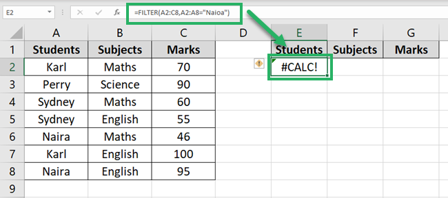
Seems like we had to write “Naira” and we mistakenly spelled it as “Naioa”. The FILTER function hence failed to find “Naioa” in the array A2:A8 🚩
This is when the FILTER function has nothing to return, and we get a #CALC error.
Now correct the spelling for Naira and rewrite the FILTER function as follows:
=FILTER(A2:C8,A2:A8=”Naira”)
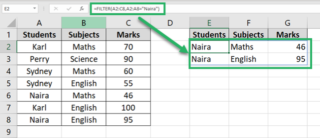
See that? As we corrected the filter criterion (the spelling of Naira), the #CALC error vanished away 🏆
Here are some quick ways to get rid of the #CALC error in Excel:
- Recheck the filter criterion supplied by you. Make sure you have used the correct spellings 📚
- Specify the [if_empty] argument for the FILTER function. This is an optional argument that tells Excel the value to be returned if nothing is found. In this case, Excel returns the [if_empty] value instead of the #CALC error if nothing is found.
Circular reference errors
A circular reference error occurs in Excel when your formula in Excel refers back to its cell (where the formula is typed) ♾
Or, when a formula refers to another cell whose results depend on this formula.
Very simply, here we are writing a PRODUCT function in Cell A1.
= PRODUCT (A2 * A1)
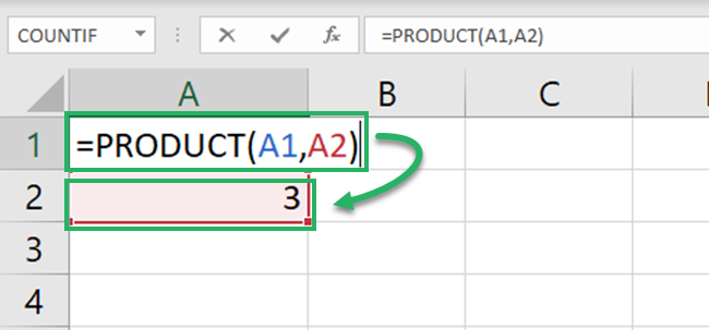
Did you note what happened? We have told Excel to multiply Cell A1 and A2. But what is Cell A1? We are yet to write the formula in Cell A1.
How can Excel multiply it by Cell A2? This is when a circular reference is created. And upon hitting Enter to process this formula, Excel returns an error message as below.

If you click on “Okay” from the dialog box above, Excel will enter into an endless loop of calculations, and you’ll probably get a zero ➿
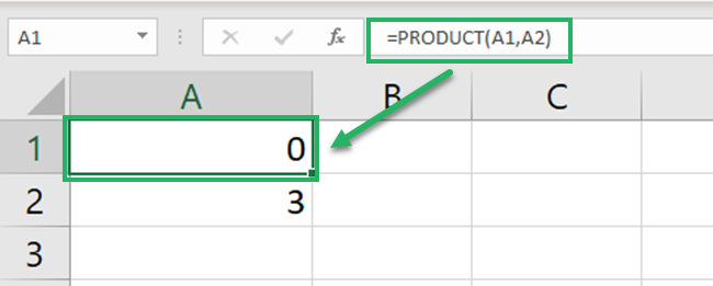
To fix circular references error in Excel, you need to find it first. For that:
- Go to the Formulas Tab > Error Checking.

- Hover over Circular References.
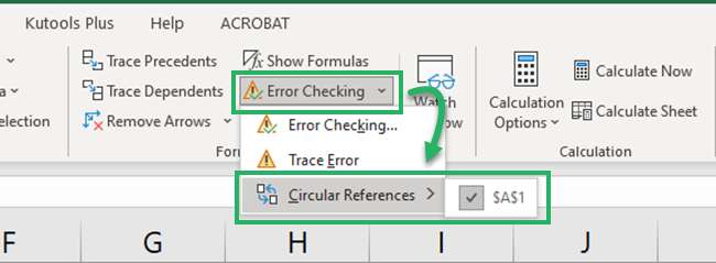
Excel will show you the cell reference and even select it for you. Once you have identified the cell causing a circular reference, delete the reference to it and that’s it 🚮
There are other ways too how you can fix the circular reference error in Excel. Learn them by reading our blog on fixing circular references in Excel.
That’s it – Now what?
The above guide makes an exhaustive list of the errors you could face in Excel. Not only the errors but their fixes too⚒
With this guide, you are all armored to sail across your number manipulation journey in Excel. And that’s not it – to become better at fixing errors in Excel, learn more about the functions in Excel.
Excel has a very long list of functions that it has to offer. But you must begin learning from some core functions. Like the VLOOKUP, SUMIF, and IF functions (some of my top favorite functions).
Want to get your hands on them already? Hop on here to enroll in my 30-minute free email course that teaches you all about these.
